Multivariate Forecasting Long Sequence Time Series with NHITS#
This notebook outlines the application of NHITS, a recently-proposed model for time series forecasting, to a collection of hourly data from California Department of Transportation, which describes the road occupancy rates measured by 862 different sensors on San Francisco Bay area freeways.
This demo uses an implementation of NHITS from the neuralforecast package. neuralforecast is a package/repository that provides implementations of several state-of-the-art deep learning-based forecasting models, namely Autoformer, Informer, NHITS and ES-RNN. Similar to PyTorch Forecasting, neuralforecast is built using PyTorch Lightning, making it easier to train in multi-GPU compute environments, out-of-the-box.
Note: neuralforecast is a relatively new package that has been gaining traction because, unlike more mature packages, it supports recent state-of-the-art methods like NHITS and Autoformer. That being said, the documentation is sparse and the package is not as mature as others we have used in other demos (PyTorch Forecasting, Prophet). In any event, neuralforecast provides a great oppurtunity to explore bleeding edge time series forecasting methods.
Environment Configuration and Package Imports#
Note for Colab users: Run the following cell to install PyTorch Forecasting. After installation completes, you will likely need to restart the Colab runtime. If this is the case, a button RESTART RUNTIME will appear at the bottom of the next cell’s output.
if 'google.colab' in str(get_ipython()):
    !pip install pytorch_lightning
    !pip install neuralforecast

if 'google.colab' in str(get_ipython()):
    from google.colab import drive
    drive.mount('/content/drive')
import warnings
import numpy as np
import pandas as pd
import matplotlib.pyplot as plt
from sklearn.metrics import mean_squared_error, mean_absolute_error, mean_absolute_percentage_error

import torch
import pytorch_lightning as pl

import neuralforecast as nf
from neuralforecast.data.datasets.epf import EPF
from pytorch_lightning.callbacks import EarlyStopping
from neuralforecast.data.tsloader import TimeSeriesLoader
from neuralforecast.experiments.utils import create_datasets
Hyperparameter Defintions#
# General Hyperparameters
VAL_PERC = .1
TEST_PERC = .1
# Model Configuration Hyperparameters
mc = {}
mc['model'] = 'n-hits' # Model Name
mc['mode'] = 'simple'
mc['activation'] = 'SELU' # Activation function


mc['n_time_in'] = 96 # Length of input sequences
mc['n_time_out'] = 96 # Length of Output Sequences
mc['n_x_hidden'] = 8 # Number of hidden output channels of exogenous_tcn and exogenous_wavenet stacks.
mc['n_s_hidden'] = 0 # Number of encoded static features

mc['stack_types'] = ['identity', 'identity', 'identity'] # List of stack types. Subset from ['seasonality', 'trend', 'identity', 'exogenous', 'exogenous_tcSubset from ['seasonality', 'trend', 'identity', 'exogenous', 'exogenous_tcn', 'exogenous_wavenet'].
mc['constant_n_blocks'] = 1 # Constant n_blocks across stacks
mc['constant_n_layers'] = 2 # Constant n_layers across stacks
mc['constant_n_mlp_units'] = 256 # Constant n_mlp_units across stacks
mc['n_pool_kernel_size'] = [4, 2, 1]  # Pooling size for input for each stack. Note that len(n_pool_kernel_size) = len(stack_types).
mc['n_freq_downsample'] = [24, 12, 1] # Downsample multiplier of output for each stack. Note that len(n_freq_downsample) = len(stack_types).
mc['pooling_mode'] = 'max' # Pooling type. An item from ['average', 'max']
mc['interpolation_mode'] = 'linear' # Interpolation function. An item from ['linear', 'nearest', 'cubic']
mc['shared_weights'] = False # If True, all blocks within each stack will share parameters.

# Optimization and regularization parameters
mc['initialization'] = 'lecun_normal'  #Initialization function. An item from ['orthogonal', 'he_uniform', 'glorot_uniform', 'glorot_normal', 'lecun_normal'].
mc['learning_rate'] = 0.001 # Learning rate between (0, 1).
mc['batch_size'] = 1 # Batch size
mc['n_windows'] = 32
mc['lr_decay'] = 0.5 # Decreasing multiplier for the learning rate.
mc['lr_decay_step_size'] = 2 # Steps between each learning rate decay.
mc['max_epochs'] = 1 # Maximum number of training epochs
mc['max_steps'] = None # Maximum number of validation epochs
mc['early_stop_patience'] = 20 #Number of consecutive violations of early stopping criteria to end training
mc['eval_freq'] = 500 # How many steps between evaluations
mc['batch_normalization'] = False # Whether perform batch normalization.
mc['dropout_prob_theta'] = 0.0 # Float between (0, 1). Dropout for Nbeats basis.
mc['dropout_prob_exogenous'] = 0.0 #
mc['weight_decay'] = 0 # L2 penalty for optimizer.
mc['loss_train'] = 'MAE' # Loss to optimize. An item from ['MAPE', 'MASE', 'SMAPE', 'MSE', 'MAE', 'QUANTILE', 'QUANTILE2'].
mc['loss_hypar'] = 0.5 # Hyperparameter for chosen loss.
mc['loss_valid'] = mc['loss_train'] #  Validation loss.  An item from ['MAPE', 'MASE', 'SMAPE', 'RMSE', 'MAE', 'QUANTILE'].
mc['random_seed'] = 1 # random_seed for pseudo random pytorch initializer and numpy random generator.

# Data Parameters
mc['idx_to_sample_freq'] = 1
mc['val_idx_to_sample_freq'] = 1
mc['n_val_weeks'] = 52
mc['normalizer_y'] = None
mc['normalizer_x'] = 'median'
mc['complete_windows'] = False # Consider only full sequences in forecasting horizon
mc['frequency'] = 'h' # Frequency of the data


# Structure of hidden layers for each stack type.
# Each internal list should contain the number of units of each hidden layer.
# Note that len(n_hidden) = len(stack_types).
mc['n_mlp_units'] = len(mc['stack_types']) * [ mc['constant_n_layers'] * [int(mc['constant_n_mlp_units'])] ]
mc['n_blocks'] =  len(mc['stack_types']) * [ mc['constant_n_blocks'] ] # Number of blocks for each stack. Note that len(n_blocks) = len(stack_types).
mc['n_layers'] =  len(mc['stack_types']) * [ mc['constant_n_layers'] ] # Number of layers for each stack type. Note that len(n_layers) = len(stack_types).

print(65*'=')
print(pd.Series(mc))
print(65*'=')
=================================================================
model                                                   n-hits
mode                                                    simple
activation                                                SELU
n_time_in                                                   96
n_time_out                                                  96
n_x_hidden                                                   8
n_s_hidden                                                   0
stack_types                     [identity, identity, identity]
constant_n_blocks                                            1
constant_n_layers                                            2
constant_n_mlp_units                                       256
n_pool_kernel_size                                   [4, 2, 1]
n_freq_downsample                                  [24, 12, 1]
pooling_mode                                               max
interpolation_mode                                      linear
shared_weights                                           False
initialization                                    lecun_normal
learning_rate                                            0.001
batch_size                                                   1
n_windows                                                   32
lr_decay                                                   0.5
lr_decay_step_size                                           2
max_epochs                                                   1
max_steps                                                 None
early_stop_patience                                         20
eval_freq                                                  500
batch_normalization                                      False
dropout_prob_theta                                         0.0
dropout_prob_exogenous                                     0.0
weight_decay                                                 0
loss_train                                                 MAE
loss_hypar                                                 0.5
loss_valid                                                 MAE
random_seed                                                  1
idx_to_sample_freq                                           1
val_idx_to_sample_freq                                       1
n_val_weeks                                                 52
normalizer_y                                              None
normalizer_x                                            median
complete_windows                                         False
frequency                                                    h
n_mlp_units               [[256, 256], [256, 256], [256, 256]]
n_blocks                                             [1, 1, 1]
n_layers                                             [2, 2, 2]
dtype: object
=================================================================
Load Data#
We start by loading the data. neuralforecast provides utilities for loading a variety of different datasets popular in the time series forecasting domain. Conveniently, the loaded data is in the format that is expected by the model that we define in the subsequent section. In particular, we call the load function with an argument specifying the dataset to load three dataframes:
Y_df: (pd.DataFrame) Target time series with columns [‘unique_id’, ‘ds’, ‘y’]X_df: (pd.DataFrame) Exogenous time series with columns [‘unique_id’, ‘ds’, ‘y’]S_df(pd.DataFrame) Static exogenous variables with columns [‘unique_id’] and static variables.
The columns referenced above are defined as follows:
unique_id: column used to identify which time series the dataframe row corresponds to. The number of unique values in the column is the number of time series in the dataset.ds: column used to identify the time stamp the dataframe row corresponds to.
In this way, a combination of unique_id and ds identify a sample in Y_df and X_df. Thus, the total number of rows they contain is the product of the unique observations in unique_id and ds. On the other hand, S_df contains a row for each exogneous variable-time series pairing. If no exogenous varables exist for any of the time sereis, S_df is None.
For datasets that are not supported out of the box for the package, we must construct these dataframes ourselves with the format specified above.
Y_df, X_df, S_df = nf.data.datasets.long_horizon.LongHorizon.load('data', 'TrafficL')
Y_df
| unique_id | ds | y | |
|---|---|---|---|
| 0 | 0 | 2016-07-01 02:00:00 | -0.711224 |
| 1 | 0 | 2016-07-01 03:00:00 | -0.672014 |
| 2 | 0 | 2016-07-01 04:00:00 | -0.724294 |
| 3 | 0 | 2016-07-01 05:00:00 | -0.725928 |
| 4 | 0 | 2016-07-01 06:00:00 | -0.721027 |
| ... | ... | ... | ... |
| 15122923 | OT | 2018-07-01 21:00:00 | 0.765917 |
| 15122924 | OT | 2018-07-01 22:00:00 | 0.389237 |
| 15122925 | OT | 2018-07-01 23:00:00 | 0.172360 |
| 15122926 | OT | 2018-07-02 00:00:00 | -0.090175 |
| 15122927 | OT | 2018-07-02 01:00:00 | -0.495391 |
15122928 rows × 3 columns
X_df
| unique_id | ds | ex_1 | ex_2 | ex_3 | ex_4 | |
|---|---|---|---|---|---|---|
| 0 | 0 | 2016-07-01 02:00:00 | -0.413043 | 0.166667 | -0.500000 | -0.00137 |
| 1 | 0 | 2016-07-01 03:00:00 | -0.369565 | 0.166667 | -0.500000 | -0.00137 |
| 2 | 0 | 2016-07-01 04:00:00 | -0.326087 | 0.166667 | -0.500000 | -0.00137 |
| 3 | 0 | 2016-07-01 05:00:00 | -0.282609 | 0.166667 | -0.500000 | -0.00137 |
| 4 | 0 | 2016-07-01 06:00:00 | -0.239130 | 0.166667 | -0.500000 | -0.00137 |
| ... | ... | ... | ... | ... | ... | ... |
| 15122923 | OT | 2018-07-01 21:00:00 | 0.413043 | 0.500000 | -0.500000 | -0.00411 |
| 15122924 | OT | 2018-07-01 22:00:00 | 0.456522 | 0.500000 | -0.500000 | -0.00411 |
| 15122925 | OT | 2018-07-01 23:00:00 | 0.500000 | 0.500000 | -0.500000 | -0.00411 |
| 15122926 | OT | 2018-07-02 00:00:00 | -0.500000 | -0.500000 | -0.466667 | -0.00137 |
| 15122927 | OT | 2018-07-02 01:00:00 | -0.456522 | -0.500000 | -0.466667 | -0.00137 |
15122928 rows × 6 columns
S_df
Y_df['ds'] = pd.to_datetime(Y_df['ds']) # Convert ds column to datetime format
X_df['ds'] = pd.to_datetime(X_df['ds']) # Convert ds column to datetime format
f_cols = X_df.drop(columns=['unique_id', 'ds']).columns.to_list()
Data Splitting#
The data is split sequentially into train, validation and test based on VAL_PERC and TEST_PERC global variables. We will withhold the last TEST_PERC of data for testing. In the code below, we are very careful to ensure that when training and validating the model, it does not have access to the withheld data.
The neuralforecast package’s function create_datasets allows us to generate a TSDataset for the train, validation and test sets by passing Y_df, X_df and S_df that we defined above. Additionally, we specify the amount of time steps we want in the validation and test datasets, ds_in_val and ds_in_test.
n_ds = Y_df["ds"].nunique()
n_val = int(VAL_PERC * n_ds)
n_test = int(TEST_PERC * n_ds)

train_dataset, val_dataset, test_dataset, scaler_y = create_datasets(mc=mc,
                                                                     S_df=None,
                                                                     Y_df=Y_df, X_df=X_df,
                                                                     f_cols=f_cols,
                                                                     ds_in_val=n_val,
                                                                     ds_in_test=n_test)
INFO:root:Train Validation splits

INFO:root:                             ds
                            min                 max
sample_mask
0           2018-02-05 22:00:00 2018-07-02 01:00:00
1           2016-07-01 02:00:00 2018-02-05 21:00:00
INFO:root:
Total data 			15122928 time stamps
Available percentage=100.0, 	15122928 time stamps
Insample  percentage=80.0, 	12099032 time stamps
Outsample percentage=20.0, 	3023896 time stamps

/ssd003/projects/aieng/public/forecasting_unified/lib/python3.8/site-packages/neuralforecast/data/tsdataset.py:208: FutureWarning: In a future version of pandas all arguments of DataFrame.drop except for the argument 'labels' will be keyword-only
  X.drop(['unique_id', 'ds'], 1, inplace=True)
INFO:root:Train Validation splits

INFO:root:                             ds
                            min                 max
sample_mask
0           2016-07-01 02:00:00 2018-07-02 01:00:00
1           2018-02-05 22:00:00 2018-04-19 23:00:00
INFO:root:
Total data 			15122928 time stamps
Available percentage=100.0, 	15122928 time stamps
Insample  percentage=10.0, 	1511948 time stamps
Outsample percentage=90.0, 	13610980 time stamps

/ssd003/projects/aieng/public/forecasting_unified/lib/python3.8/site-packages/neuralforecast/data/tsdataset.py:208: FutureWarning: In a future version of pandas all arguments of DataFrame.drop except for the argument 'labels' will be keyword-only
  X.drop(['unique_id', 'ds'], 1, inplace=True)
INFO:root:Train Validation splits

INFO:root:                             ds
                            min                 max
sample_mask
0           2016-07-01 02:00:00 2018-04-19 23:00:00
1           2018-04-20 00:00:00 2018-07-02 01:00:00
INFO:root:
Total data 			15122928 time stamps
Available percentage=100.0, 	15122928 time stamps
Insample  percentage=10.0, 	1511948 time stamps
Outsample percentage=90.0, 	13610980 time stamps

/ssd003/projects/aieng/public/forecasting_unified/lib/python3.8/site-packages/neuralforecast/data/tsdataset.py:208: FutureWarning: In a future version of pandas all arguments of DataFrame.drop except for the argument 'labels' will be keyword-only
  X.drop(['unique_id', 'ds'], 1, inplace=True)
Defining Dataloader#
The neural forecasting package defines its own dataloader TimeSeriesLoader. Similar to a regular PyTorch dataloader, we pass a dataset, batch size and other paraneters that inform how each batch of data is loaded.
train_loader = TimeSeriesLoader(dataset=train_dataset,
                                batch_size=int(mc['batch_size']),
                                n_windows=mc['n_windows'],
                                shuffle=True)

val_loader = TimeSeriesLoader(dataset=val_dataset,
                              batch_size=int(mc['batch_size']),
                              shuffle=False)

test_loader = TimeSeriesLoader(dataset=test_dataset,
                               batch_size=int(mc['batch_size']),
                               shuffle=False)
Model#
NHITS Overview#

NHITS is a popular deep learning based approach to time series forecasting. In particualr, NHITS adapts the NBEATS architecture to perform long sequence time series forecasting (LSTF); a task where the length of the input and output sequence are large. NHITS learns a global model from historical data of one or more time series. Thus, although the input and output space is univariate, NHITS can be used to jointly model a set of related time series. The architecture consists of deep stacks of fully connected layers connected with forward and backward residual links. The forwad links aggregate partial forecast to yield final forecast. Alternatively, backward links subtract out input signal corresponding to already predicted partial forecast from input prior to being passed to the next stack. NHITS builds on NBEATS by enhancing its input decomposition via multi-rate data sampling and its output synthesizer via multi-scale interpolation. This increases both the accuracy and computational efficiency of the approach in the LSTF setting.
Some additional features of NHITS include:
Interpretability: Allows for hierarchical decomposition of a forecasts into trend and seasonal components which enhances interpretability.
Ensembling: Ensembles models fit with different loss functions and time horizons. The final prediction is mean of models in ensemble.
Efficient: Avoids the use of recurrent structute and predicts entire ouput sequence in single forward pass.
Model Definition#
Using the neuralforecast package, an NHITS model can be initialized using the NHITS class. This returns a Pytorch Lighnting model that we will subsequently train and evaluate. There is a large amount of parameters involved in the definition, most of which can stay consistent accross datasets. Some of the arguments that may vary include:
n_time_in: (int) The length of sequences input to the model.n_time_out: (int) The length of the sequences output by the model.n_x: (int) The number of exogenous time series. This equals the number of features included inX_df.n_s: (int) The number of static exogenous variables. This equals the number of features included inS_df.frequency: (string) The frequency of the observations. (hourly:h, daily:d)
For additional details in regards to the NHITS class, consult the neuralforecast documentation. Values of model hyperparameters with corresponding defintions is available above in the Hyperparameter Defintions section.
mc['n_x'], mc['n_s'] = train_dataset.get_n_variables()

model = nf.models.nhits.nhits.NHITS(n_time_in=int(mc['n_time_in']),
              n_time_out=int(mc['n_time_out']),
              n_x=mc['n_x'],
              n_s=mc['n_s'],
              n_s_hidden=int(mc['n_s_hidden']),
              n_x_hidden=int(mc['n_x_hidden']),
              shared_weights=mc['shared_weights'],
              initialization=mc['initialization'],
              activation=mc['activation'],
              stack_types=mc['stack_types'],
              n_blocks=mc['n_blocks'],
              n_layers=mc['n_layers'],
              n_mlp_units=mc['n_mlp_units'],
              n_pool_kernel_size=mc['n_pool_kernel_size'],
              n_freq_downsample=mc['n_freq_downsample'],
              pooling_mode=mc['pooling_mode'],
              interpolation_mode=mc['interpolation_mode'],
              batch_normalization = mc['batch_normalization'],
              dropout_prob_theta=mc['dropout_prob_theta'],
              learning_rate=float(mc['learning_rate']),
              lr_decay=float(mc['lr_decay']),
              lr_decay_step_size=float(mc['lr_decay_step_size']),
              weight_decay=mc['weight_decay'],
              loss_train=mc['loss_train'],
              loss_hypar=float(mc['loss_hypar']),
              loss_valid=mc['loss_valid'],
              frequency=mc['frequency'],
              random_seed=int(mc['random_seed']))
Training and Validation#
We first define a pytorch lighting trainer which encapsulates the training process and allows us to easily implement a training and validation loop with the specified parameters. The arguments to the trainer include:
max_epochs: (Optional[int]) – Stop training once this number of epochs is reached.callbacks: (Union[List[Callback], Callback, None]) – Add a callback or list of callbacks.
Subsequently, we can use the fit method of the trainer with the net, train_dataloader and val_dataloader to perform the training and validation loop.
For more information regarding the pl.Trainer class, consult the PyTorch Lightning documentation.
# Set random seed
pl.seed_everything(42)

# Define early stopping criteria
early_stopping = EarlyStopping(monitor="val_loss",
                               min_delta=1e-4,
                               patience=mc['early_stop_patience'],
                               verbose=False,
                               mode="min")

# Init pytorch lightning trainer
trainer = pl.Trainer(accelerator="gpu",
                     devices=1,
                     max_epochs=mc['max_epochs'],
                     gradient_clip_val=1.0,
                     progress_bar_refresh_rate=10,
                     log_every_n_steps=500,
                     check_val_every_n_epoch=1,
                     callbacks=[early_stopping])

# Train and Validate Model
trainer.fit(model, train_loader, val_loader)
Global seed set to 42
/ssd003/projects/aieng/public/forecasting_unified/lib/python3.8/site-packages/pytorch_lightning/trainer/connectors/callback_connector.py:90: LightningDeprecationWarning: Setting `Trainer(progress_bar_refresh_rate=10)` is deprecated in v1.5 and will be removed in v1.7. Please pass `pytorch_lightning.callbacks.progress.TQDMProgressBar` with `refresh_rate` directly to the Trainer's `callbacks` argument instead. Or, to disable the progress bar pass `enable_progress_bar = False` to the Trainer.
  rank_zero_deprecation(
GPU available: True, used: True
TPU available: False, using: 0 TPU cores
IPU available: False, using: 0 IPUs
LOCAL_RANK: 0 - CUDA_VISIBLE_DEVICES: [0]
Set SLURM handle signals.

  | Name  | Type   | Params
---------------------------------
0 | model | _NHITS | 932 K
---------------------------------
932 K     Trainable params
0         Non-trainable params
932 K     Total params
3.731     Total estimated model params size (MB)
/ssd003/projects/aieng/public/forecasting_unified/lib/python3.8/site-packages/pytorch_lightning/trainer/data_loading.py:132: UserWarning: The dataloader, val_dataloader 0, does not have many workers which may be a bottleneck. Consider increasing the value of the `num_workers` argument` (try 32 which is the number of cpus on this machine) in the `DataLoader` init to improve performance.
  rank_zero_warn(
/ssd003/projects/aieng/public/forecasting_unified/lib/python3.8/site-packages/torch/nn/functional.py:3631: UserWarning: Default upsampling behavior when mode=linear is changed to align_corners=False since 0.4.0. Please specify align_corners=True if the old behavior is desired. See the documentation of nn.Upsample for details.
  warnings.warn(
Global seed set to 42
/ssd003/projects/aieng/public/forecasting_unified/lib/python3.8/site-packages/pytorch_lightning/trainer/data_loading.py:132: UserWarning: The dataloader, train_dataloader, does not have many workers which may be a bottleneck. Consider increasing the value of the `num_workers` argument` (try 32 which is the number of cpus on this machine) in the `DataLoader` init to improve performance.
  rank_zero_warn(
Test#
Inference#
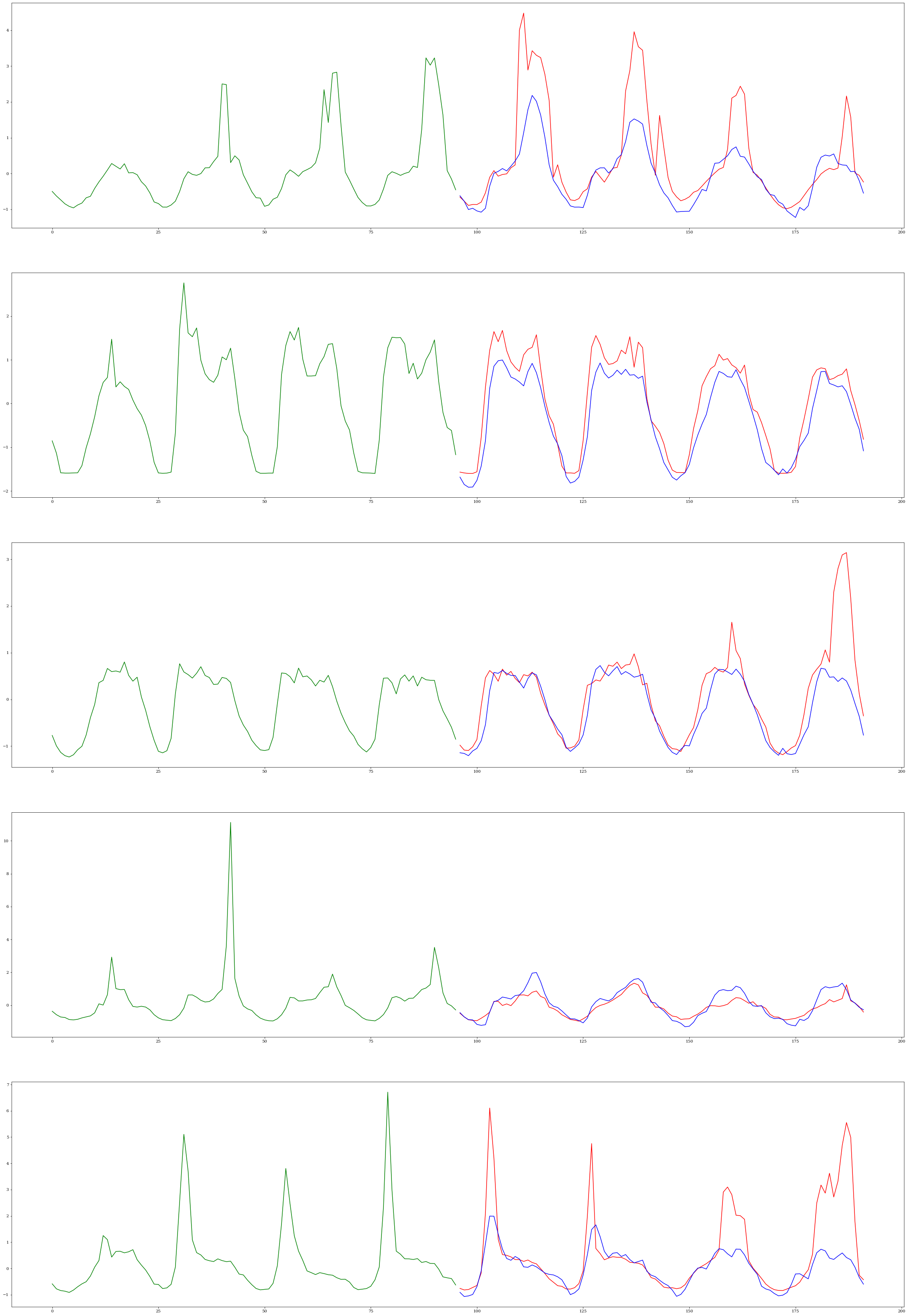
We can obtain the predictions of the trained model on the test samples using the predict method of the trainer object. This will output a list the same length as the number of time series. Each entry in this list (ie outputs[0]) is a list itself where the first item (ie outputs[0][0]) is the ground truth and the second item (ie outputs[0][1]) is the prediction.
# Obtain Predictions on Test Set
model.return_decomposition = False
outputs = trainer.predict(model, test_loader)
LOCAL_RANK: 0 - CUDA_VISIBLE_DEVICES: [0]
/ssd003/projects/aieng/public/forecasting_unified/lib/python3.8/site-packages/neuralforecast/data/tsloader.py:46: UserWarning: This class wraps the pytorch `DataLoader` with a special collate function. If you want to use yours simply use `DataLoader`. Removing collate_fn
  warnings.warn(
/ssd003/projects/aieng/public/forecasting_unified/lib/python3.8/site-packages/pytorch_lightning/trainer/data_loading.py:132: UserWarning: The dataloader, predict_dataloader 0, does not have many workers which may be a bottleneck. Consider increasing the value of the `num_workers` argument` (try 32 which is the number of cpus on this machine) in the `DataLoader` init to improve performance.
  rank_zero_warn(
Visualize Predictions#
With the trained model from the previous step, we can apply it to the test set to get an unbias estimate of the models performance. Additionally, we can visualize the results to build some intuition about the forecasts being generated.
input_list, gt_list = [], []
for d in test_loader:
    Y = d["Y"]
    inp = Y[:, :mc['n_time_in']]
    input_list.append(inp)
n_samples = 5
ss_indices = np.random.choice((len(outputs)), n_samples, replace=False).tolist()

f, axarr = plt.subplots(n_samples, 1, figsize=(40, 60))

for i, ss_ind in enumerate(ss_indices):
    inp = input_list[ss_ind][0, :].cpu().numpy()

    out1 = outputs[ss_ind][0][0, :].cpu().numpy()
    out2 = outputs[ss_ind][1][0, :].cpu().numpy()

    inp_index = [j for j in range(mc['n_time_in'])]
    out_index = [j for j in range(mc['n_time_in'], mc['n_time_out'] + mc['n_time_out'])]

    axarr[i].plot(inp_index, inp, c="green")
    axarr[i].plot(out_index, out1, c="red")
    axarr[i].plot(out_index, out2, c="blue")
Quantitative Resutls#
To assess the performance of NHITS on the dataset, we calculate its performance on the test set using a set of metrics that are commonly used in time series forecasting. The metrics include Mean Absolute Error (MAE) and Mean Squared Error (MSE).
# Aggregate list of ground truth and prediction series in to lists
true_list = [output[0] for output in outputs]
pred_list = [output[1] for output in outputs]

# Stack lists into tensors along the sample/batch dimension
trues = torch.concat(true_list, dim=0)
preds = torch.concat(pred_list, dim=0)

# Calculate Losses
mse = mean_squared_error(trues.cpu().numpy(), preds.cpu().numpy())
mae = mean_absolute_error(trues.cpu().numpy(), preds.cpu().numpy())

print(f"MSE: {mse} MAE: {mae}")
MSE: 0.644439697265625 MAE: 0.41899624466896057