M5 Data Preparation

This notebook helps with loading and transforming the M5 dataset into higher-level, aggregate time series. M5, by default, is provided as a set of 30,490 individual time series. These correspond to individual product sales figures at individual Walmart stores. These time series can be naturally aggregated according to a hierarchy:

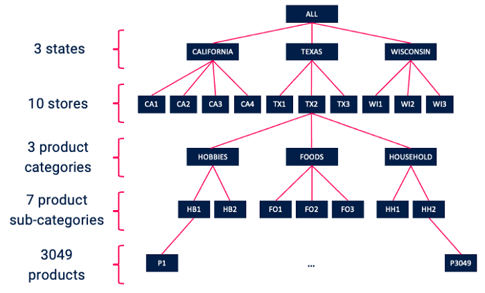
As we can see, the 30,490 time series correspond to sales figures for 3049 individual products across 10 stores. The products each belong to one of three product categories (Hobbies, Foods, and Household), which can be further broken down into a total of 7 product subcategories. The 10 stores each belong to one of three states (California, Texas, and Wisconsin).

Other information are also provided as part of the M5 dataset, including product sell prices and a calendar of important events (e.g. holidays, relevant dates for nutrition assistance programs).

The following code has been adapted from this repository for the official 2nd place M5 solution.

Load data

import pandas as pd

m5_input_path = "/ssd003/projects/forecasting_bootcamp/bootcamp_datasets/m5-forecasting-accuracy"
sell_price = pd.read_csv(f'{m5_input_path}/sell_prices.csv')
calendar = pd.read_csv(f'{m5_input_path}/calendar.csv')
train = pd.read_csv(f'{m5_input_path}/sales_train_evaluation.csv').set_index('id')
sample_sub = pd.read_csv(f'{m5_input_path}/sample_submission.csv')

Build aggregate dataset

# Get column groups
cat_cols = ['item_id', 'dept_id', 'cat_id', 'store_id', 'state_id']
ts_cols = [col for col in train.columns if col not in cat_cols]
ts_dict = {t: int(t[2:]) for t in ts_cols}

# Describe data
print('  unique forecasts: %i' % train.shape[0])
for col in cat_cols:
    print('   N_unique %s: %i' % (col, train[col].nunique()))

  unique forecasts: 30490
   N_unique item_id: 3049
   N_unique dept_id: 7
   N_unique cat_id: 3
   N_unique store_id: 10
   N_unique state_id: 3

%%time
# 1. All products, all stores, all states (1 series)
all_sales = pd.DataFrame(train[ts_cols].sum()).transpose()
all_sales['id_str'] = 'all'
all_sales = all_sales[ ['id_str'] +  [c for c in all_sales if c not in ['id_str']] ]
all_sales

CPU times: user 133 ms, sys: 140 ms, total: 273 ms
Wall time: 269 ms

	id_str	d_1	d_2	d_3	d_4	d_5	d_6	d_7	d_8	d_9	...	d_1932	d_1933	d_1934	d_1935	d_1936	d_1937	d_1938	d_1939	d_1940	d_1941
0	all	32631	31749	23783	25412	19146	29211	28010	37932	32736	...	44073	54308	59921	42362	38777	37096	36963	42552	51518	54338

1 rows × 1942 columns

%%time
# 2. All products by state (3 series)
state_sales = train.groupby('state_id',as_index=False)[ts_cols].sum()
state_sales['id_str'] = state_sales['state_id'] 
state_sales = state_sales[ ['id_str'] +  [c for c in state_sales if c not in ['id_str']] ]
state_sales = state_sales.drop(['state_id'],axis=1)
state_sales

CPU times: user 734 ms, sys: 813 ms, total: 1.55 s
Wall time: 1.58 s

	id_str	d_1	d_2	d_3	d_4	d_5	d_6	d_7	d_8	d_9	...	d_1932	d_1933	d_1934	d_1935	d_1936	d_1937	d_1938	d_1939	d_1940	d_1941
0	CA	14195	13805	10108	11047	9925	11322	12251	16610	14696	...	18471	23037	24704	17721	16150	15678	16297	17430	23103	24644
1	TX	9438	9630	6778	7381	5912	9006	6226	9440	9376	...	12320	12366	16249	12228	11370	10375	9162	12303	13681	14815
2	WI	8998	8314	6897	6984	3309	8883	9533	11882	8664	...	13282	18905	18968	12413	11257	11043	11504	12819	14734	14879

3 rows × 1942 columns

%%time
# 3. All products by store (10 series)
store_sales = train.groupby('store_id',as_index=False)[ts_cols].sum()
store_sales['id_str'] = store_sales['store_id'] 
store_sales = store_sales[ ['id_str'] +  [c for c in store_sales if c not in ['id_str']] ]
store_sales = store_sales.drop(['store_id'],axis=1)
store_sales

CPU times: user 735 ms, sys: 1.87 s, total: 2.61 s
Wall time: 2.6 s

	id_str	d_1	d_2	d_3	d_4	d_5	d_6	d_7	d_8	d_9	...	d_1932	d_1933	d_1934	d_1935	d_1936	d_1937	d_1938	d_1939	d_1940	d_1941
0	CA_1	4337	4155	2816	3051	2630	3276	3450	5437	4340	...	4951	6245	6707	4568	3949	3995	4136	4433	5764	6289
1	CA_2	3494	3046	2121	2324	1942	2288	2629	3729	2957	...	4839	6507	6710	4238	3963	3789	4037	4751	7120	6614
2	CA_3	4739	4827	3785	4232	3817	4369	4703	5456	5581	...	6046	7029	7969	5891	5523	5375	5580	5542	7073	8144
3	CA_4	1625	1777	1386	1440	1536	1389	1469	1988	1818	...	2635	3256	3318	3024	2715	2519	2544	2704	3146	3597
4	TX_1	2556	2687	1822	2258	1694	2734	1691	2820	2887	...	3610	3787	5000	3708	3310	3147	2748	3664	4167	4624
5	TX_2	3852	3937	2731	2954	2492	3439	2588	3772	3657	...	4415	4424	5866	4179	4008	3518	3126	4249	4802	5217
6	TX_3	3030	3006	2225	2169	1726	2833	1947	2848	2832	...	4295	4155	5383	4341	4052	3710	3288	4390	4712	4974
7	WI_1	2704	2194	1562	1251	2	2049	2815	3248	1674	...	3978	5527	5488	3505	3323	3242	3478	3813	5002	5054
8	WI_2	2256	1922	2018	2522	1175	2244	2232	2643	2140	...	5317	7704	7586	5011	4628	4533	4628	4880	5213	5068
9	WI_3	4038	4198	3317	3211	2132	4590	4486	5991	4850	...	3987	5674	5894	3897	3306	3268	3398	4126	4519	4757

10 rows × 1942 columns

%%time
# 4. All products by category (3 series)
cat_sales = train.groupby('cat_id',as_index=False)[ts_cols].sum()
cat_sales['id_str'] = cat_sales['cat_id'] 
cat_sales = cat_sales[ ['id_str'] +  [c for c in cat_sales if c not in ['id_str']] ]
cat_sales = cat_sales.drop(['cat_id'],axis=1)
cat_sales

CPU times: user 725 ms, sys: 279 ms, total: 1 s
Wall time: 1 s

	id_str	d_1	d_2	d_3	d_4	d_5	d_6	d_7	d_8	d_9	...	d_1932	d_1933	d_1934	d_1935	d_1936	d_1937	d_1938	d_1939	d_1940	d_1941
0	FOODS	23178	22758	17174	18878	14603	22093	20490	27751	24862	...	30107	36576	41447	29158	26148	24790	24737	28136	33599	35967
1	HOBBIES	3764	3357	2682	2669	1814	3220	2944	3986	2899	...	3871	4893	5016	3528	3629	3740	3475	4143	5333	5280
2	HOUSEHOLD	5689	5634	3927	3865	2729	3898	4576	6195	4975	...	10095	12839	13458	9676	9000	8566	8751	10273	12586	13091

3 rows × 1942 columns

%%time
# 5. All products by department (7 series)
dept_sales = train.groupby('dept_id',as_index=False)[ts_cols].sum()
dept_sales['id_str'] = dept_sales['dept_id'] 
dept_sales = dept_sales[ ['id_str'] +  [c for c in dept_sales if c not in ['id_str']] ]
dept_sales = dept_sales.drop(['dept_id'],axis=1)
dept_sales

CPU times: user 722 ms, sys: 491 ms, total: 1.21 s
Wall time: 1.21 s

	id_str	d_1	d_2	d_3	d_4	d_5	d_6	d_7	d_8	d_9	...	d_1932	d_1933	d_1934	d_1935	d_1936	d_1937	d_1938	d_1939	d_1940	d_1941
0	FOODS_1	2343	2216	1657	1508	1209	1897	1903	2235	1925	...	4130	4257	4225	3264	3119	3073	3251	3735	4195	4031
1	FOODS_2	4094	4209	3174	3606	2869	4375	3349	4384	4273	...	5842	7563	9069	6226	5311	4648	4551	4815	5940	6535
2	FOODS_3	16741	16333	12343	13764	10525	15821	15238	21132	18664	...	20135	24756	28153	19668	17718	17069	16935	19586	23464	25401
3	HOBBIES_1	3610	3172	2497	2531	1714	3133	2855	3831	2741	...	3422	4414	4464	3109	3142	3291	3027	3761	4832	4720
4	HOBBIES_2	154	185	185	138	100	87	89	155	158	...	449	479	552	419	487	449	448	382	501	560
5	HOUSEHOLD_1	4105	3858	2827	2732	1802	2664	3161	4334	3494	...	7936	10042	10572	7609	6999	6641	6759	7974	9668	10165
6	HOUSEHOLD_2	1584	1776	1100	1133	927	1234	1415	1861	1481	...	2159	2797	2886	2067	2001	1925	1992	2299	2918	2926

7 rows × 1942 columns

## TOP LEVEL aggregates + TOTAL
all_aggregates = pd.concat([all_sales,state_sales,store_sales,cat_sales,dept_sales],ignore_index=True)
all_aggregates

	id_str	d_1	d_2	d_3	d_4	d_5	d_6	d_7	d_8	d_9	...	d_1932	d_1933	d_1934	d_1935	d_1936	d_1937	d_1938	d_1939	d_1940	d_1941
0	all	32631	31749	23783	25412	19146	29211	28010	37932	32736	...	44073	54308	59921	42362	38777	37096	36963	42552	51518	54338
1	CA	14195	13805	10108	11047	9925	11322	12251	16610	14696	...	18471	23037	24704	17721	16150	15678	16297	17430	23103	24644
2	TX	9438	9630	6778	7381	5912	9006	6226	9440	9376	...	12320	12366	16249	12228	11370	10375	9162	12303	13681	14815
3	WI	8998	8314	6897	6984	3309	8883	9533	11882	8664	...	13282	18905	18968	12413	11257	11043	11504	12819	14734	14879
4	CA_1	4337	4155	2816	3051	2630	3276	3450	5437	4340	...	4951	6245	6707	4568	3949	3995	4136	4433	5764	6289
5	CA_2	3494	3046	2121	2324	1942	2288	2629	3729	2957	...	4839	6507	6710	4238	3963	3789	4037	4751	7120	6614
6	CA_3	4739	4827	3785	4232	3817	4369	4703	5456	5581	...	6046	7029	7969	5891	5523	5375	5580	5542	7073	8144
7	CA_4	1625	1777	1386	1440	1536	1389	1469	1988	1818	...	2635	3256	3318	3024	2715	2519	2544	2704	3146	3597
8	TX_1	2556	2687	1822	2258	1694	2734	1691	2820	2887	...	3610	3787	5000	3708	3310	3147	2748	3664	4167	4624
9	TX_2	3852	3937	2731	2954	2492	3439	2588	3772	3657	...	4415	4424	5866	4179	4008	3518	3126	4249	4802	5217
10	TX_3	3030	3006	2225	2169	1726	2833	1947	2848	2832	...	4295	4155	5383	4341	4052	3710	3288	4390	4712	4974
11	WI_1	2704	2194	1562	1251	2	2049	2815	3248	1674	...	3978	5527	5488	3505	3323	3242	3478	3813	5002	5054
12	WI_2	2256	1922	2018	2522	1175	2244	2232	2643	2140	...	5317	7704	7586	5011	4628	4533	4628	4880	5213	5068
13	WI_3	4038	4198	3317	3211	2132	4590	4486	5991	4850	...	3987	5674	5894	3897	3306	3268	3398	4126	4519	4757
14	FOODS	23178	22758	17174	18878	14603	22093	20490	27751	24862	...	30107	36576	41447	29158	26148	24790	24737	28136	33599	35967
15	HOBBIES	3764	3357	2682	2669	1814	3220	2944	3986	2899	...	3871	4893	5016	3528	3629	3740	3475	4143	5333	5280
16	HOUSEHOLD	5689	5634	3927	3865	2729	3898	4576	6195	4975	...	10095	12839	13458	9676	9000	8566	8751	10273	12586	13091
17	FOODS_1	2343	2216	1657	1508	1209	1897	1903	2235	1925	...	4130	4257	4225	3264	3119	3073	3251	3735	4195	4031
18	FOODS_2	4094	4209	3174	3606	2869	4375	3349	4384	4273	...	5842	7563	9069	6226	5311	4648	4551	4815	5940	6535
19	FOODS_3	16741	16333	12343	13764	10525	15821	15238	21132	18664	...	20135	24756	28153	19668	17718	17069	16935	19586	23464	25401
20	HOBBIES_1	3610	3172	2497	2531	1714	3133	2855	3831	2741	...	3422	4414	4464	3109	3142	3291	3027	3761	4832	4720
21	HOBBIES_2	154	185	185	138	100	87	89	155	158	...	449	479	552	419	487	449	448	382	501	560
22	HOUSEHOLD_1	4105	3858	2827	2732	1802	2664	3161	4334	3494	...	7936	10042	10572	7609	6999	6641	6759	7974	9668	10165
23	HOUSEHOLD_2	1584	1776	1100	1133	927	1234	1415	1861	1481	...	2159	2797	2886	2067	2001	1925	1992	2299	2918	2926

24 rows × 1942 columns

main_df = all_aggregates.set_index('id_str').T
main_df['date'] = calendar[['d', 'date']].set_index('d')['date']
main_df = main_df.set_index('date')
main_df.index = pd.DatetimeIndex(main_df.index)
main_df

id_str	all	CA	TX	WI	CA_1	CA_2	CA_3	CA_4	TX_1	TX_2	...	FOODS	HOBBIES	HOUSEHOLD	FOODS_1	FOODS_2	FOODS_3	HOBBIES_1	HOBBIES_2	HOUSEHOLD_1	HOUSEHOLD_2
date
2011-01-29	32631	14195	9438	8998	4337	3494	4739	1625	2556	3852	...	23178	3764	5689	2343	4094	16741	3610	154	4105	1584
2011-01-30	31749	13805	9630	8314	4155	3046	4827	1777	2687	3937	...	22758	3357	5634	2216	4209	16333	3172	185	3858	1776
2011-01-31	23783	10108	6778	6897	2816	2121	3785	1386	1822	2731	...	17174	2682	3927	1657	3174	12343	2497	185	2827	1100
2011-02-01	25412	11047	7381	6984	3051	2324	4232	1440	2258	2954	...	18878	2669	3865	1508	3606	13764	2531	138	2732	1133
2011-02-02	19146	9925	5912	3309	2630	1942	3817	1536	1694	2492	...	14603	1814	2729	1209	2869	10525	1714	100	1802	927
...	...	...	...	...	...	...	...	...	...	...	...	...	...	...	...	...	...	...	...	...	...
2016-05-18	37096	15678	10375	11043	3995	3789	5375	2519	3147	3518	...	24790	3740	8566	3073	4648	17069	3291	449	6641	1925
2016-05-19	36963	16297	9162	11504	4136	4037	5580	2544	2748	3126	...	24737	3475	8751	3251	4551	16935	3027	448	6759	1992
2016-05-20	42552	17430	12303	12819	4433	4751	5542	2704	3664	4249	...	28136	4143	10273	3735	4815	19586	3761	382	7974	2299
2016-05-21	51518	23103	13681	14734	5764	7120	7073	3146	4167	4802	...	33599	5333	12586	4195	5940	23464	4832	501	9668	2918
2016-05-22	54338	24644	14815	14879	6289	6614	8144	3597	4624	5217	...	35967	5280	13091	4031	6535	25401	4720	560	10165	2926

1941 rows × 24 columns

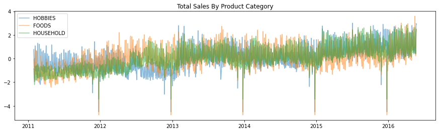
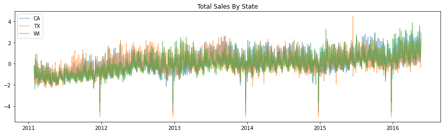
Aggregate time series visualization

Visualize data using different aggregation levels, e.g. by product category and by state. Scale the data to help vizualize differences in patterns.

import matplotlib.pyplot as plt
from sklearn.preprocessing import scale

fig, ax = plt.subplots(figsize=(15,4))
ax.plot(main_df.index, scale(main_df['HOBBIES']), label='HOBBIES', alpha=0.5)
ax.plot(main_df.index, scale(main_df['FOODS']), label='FOODS', alpha=0.5)
ax.plot(main_df.index, scale(main_df['HOUSEHOLD']), label='HOUSEHOLD', alpha=0.5)
plt.legend()
plt.title("Total Sales By Product Category")

Text(0.5, 1.0, 'Total Sales By Product Category')

fig, ax = plt.subplots(figsize=(15,4))
ax.plot(main_df.index, scale(main_df['CA']), label='CA', alpha=0.5)
ax.plot(main_df.index, scale(main_df['TX']), label='TX', alpha=0.5)
ax.plot(main_df.index, scale(main_df['WI']), label='WI', alpha=0.5)
plt.legend()
plt.title("Total Sales By State")

Text(0.5, 1.0, 'Total Sales By State')

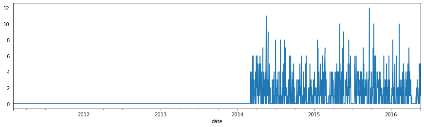
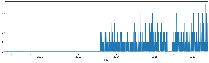
Visualize individual product sales time series.

product_sales = train[ts_cols].T
product_sales['date'] = calendar[['d', 'date']].set_index('d')['date']
product_sales = product_sales.set_index('date')
product_sales.index = pd.DatetimeIndex(product_sales.index)
product_sales

id	HOBBIES_1_001_CA_1_evaluation	HOBBIES_1_002_CA_1_evaluation	HOBBIES_1_003_CA_1_evaluation	HOBBIES_1_004_CA_1_evaluation	HOBBIES_1_005_CA_1_evaluation	HOBBIES_1_006_CA_1_evaluation	HOBBIES_1_007_CA_1_evaluation	HOBBIES_1_008_CA_1_evaluation	HOBBIES_1_009_CA_1_evaluation	HOBBIES_1_010_CA_1_evaluation	...	FOODS_3_818_WI_3_evaluation	FOODS_3_819_WI_3_evaluation	FOODS_3_820_WI_3_evaluation	FOODS_3_821_WI_3_evaluation	FOODS_3_822_WI_3_evaluation	FOODS_3_823_WI_3_evaluation	FOODS_3_824_WI_3_evaluation	FOODS_3_825_WI_3_evaluation	FOODS_3_826_WI_3_evaluation	FOODS_3_827_WI_3_evaluation
date
2011-01-29	0	0	0	0	0	0	0	12	2	0	...	0	14	1	0	4	0	0	0	0	0
2011-01-30	0	0	0	0	0	0	0	15	0	0	...	0	11	1	0	4	0	0	6	0	0
2011-01-31	0	0	0	0	0	0	0	0	7	1	...	0	5	1	0	2	2	0	0	0	0
2011-02-01	0	0	0	0	0	0	0	0	3	0	...	0	6	1	0	5	2	0	2	0	0
2011-02-02	0	0	0	0	0	0	0	0	0	0	...	0	5	1	0	2	0	0	2	0	0
...	...	...	...	...	...	...	...	...	...	...	...	...	...	...	...	...	...	...	...	...	...
2016-05-18	0	0	0	1	0	0	1	5	0	1	...	3	6	3	0	0	1	0	1	0	0
2016-05-19	3	0	2	3	0	0	0	4	0	1	...	1	4	3	1	2	0	1	0	1	2
2016-05-20	3	0	3	0	2	5	1	1	0	0	...	3	4	3	1	1	0	0	1	1	2
2016-05-21	0	0	0	2	1	2	1	40	1	0	...	0	1	0	0	3	1	1	0	1	5
2016-05-22	1	0	1	6	0	0	0	32	0	1	...	0	1	1	4	4	1	0	2	0	1

1941 rows × 30490 columns

product_sales['HOBBIES_1_001_CA_1_evaluation'].plot(figsize=(15,4))

<AxesSubplot:xlabel='date'>

product_sales['FOODS_3_827_WI_3_evaluation'].plot(figsize=(15,4))

<AxesSubplot:xlabel='date'>