Multivariate Forecasting Long Sequence Time Series with Autoformer#
This notebook outlines the application of Autoformer, a recently-proposed model for time series forecasting, to a collection of hourly data from California Department of Transportation, which describes the road occupancy rates measured by 862 different sensors on San Francisco Bay area freeways.
This demo uses an implementation of NHTIS from the neuralforecast package. neuralforecast is a package/repository that provides implementations of several state-of-the-art deep learning-based forecasting models, namely Autoformer, Informer, NHITS and ES-RNN. Similar to PyTorch Forecasting, neuralforecast is built using PyTorch Lightning, making it easier to train in multi-GPU compute environments, out-of-the-box.
Note: neuralforecast is a relatively new package that has been gaining traction because, unlike more mature packages, it supports recent state-of-the-art methods like NHITS and Autoformer. That being said, the documentation is sparse and the package is not as mature as others we have used in other demos (PyTorch Forecasting, Prophet). In any event, neuralforecast provides a great oppurtunity to explore bleeding edge time series forecasting methods.
Environment Configuration and Package Imports#
Note for Colab users: Run the following cell to install PyTorch Forecasting. After installation completes, you will likely need to restart the Colab runtime. If this is the case, a button RESTART RUNTIME will appear at the bottom of the next cell’s output.
if 'google.colab' in str(get_ipython()):
    !pip install pytorch_lightning
    !pip install neuralforecast
import warnings
import numpy as np
import pandas as pd
import matplotlib.pyplot as plt
from sklearn.metrics import mean_squared_error, mean_absolute_error, mean_absolute_percentage_error

import torch
from torch.utils.data import DataLoader

import pytorch_lightning as pl

import neuralforecast as nf
from neuralforecast.data.datasets.epf import EPF
from pytorch_lightning.callbacks import EarlyStopping
from neuralforecast.data.tsloader import TimeSeriesLoader
from neuralforecast.experiments.utils import create_datasets
from neuralforecast.data.tsdataset import IterateWindowsDataset
warnings.filterwarnings("ignore") # Comment out
Hyperparameter Definitions#
VAL_PERC = .1
TEST_PERC = .1
N_TIME_SERIES = 862
mc_model = {}

mc_model['seq_len'] = 96 # Input sequence size.
mc_model['label_len'] = 96 // 2 # Label sequence size. (Input buffer length for decoder)
mc_model['pred_len'] = 96 # Prediction sequence size.
mc_model['output_attention'] = False # If true use output attention for Transformer model.
mc_model['enc_in'] = N_TIME_SERIES #  Number of encoders in data embedding layers.
mc_model['dec_in'] = N_TIME_SERIES #  Number of decoders in data embedding layers.
mc_model['d_model'] = 512 #  Number of nodes for embedding layers.
mc_model['c_out'] = N_TIME_SERIES # Number of output nodes in projection layer.
mc_model['embed'] = 'timeF' #  Type of embedding layers.
mc_model['freq'] = 'h' # Frequency for embedding layers.
mc_model['dropout'] = 0.05 # Float between (0, 1). Dropout for Transformer.
mc_model['factor'] = 1 # Factor for attention layer.
mc_model['n_heads'] = 8 #  Number of heads in attention layer.
mc_model['d_ff'] = 2_048 #  Number of inputs in encoder layers.
mc_model['moving_avg'] = 25  #  Moving average for encoder and decoder layers.
mc_model['activation'] = 'gelu' #  Activation function for encoder layer.
mc_model['e_layers'] = 2 # Number of encoder layers.
mc_model['d_layers'] = 1 # Number of decoder layers.
mc_model['loss_train'] = 'MAE' # Loss to optimize. An item from ['MAPE', 'MASE', 'SMAPE', 'MSE', 'MAE', 'QUANTILE', 'QUANTILE2'].
mc_model['loss_hypar'] = 0.5 # Hyperparameter for chosen loss.
mc_model['loss_valid'] = 'MAE'# Validation loss.An item from ['MAPE', 'MASE', 'SMAPE', 'RMSE', 'MAE', 'QUANTILE'].
mc_model['learning_rate'] = 0.001 # Learning rate between (0, 1).
mc_model['lr_decay'] = 0.5 # Decreasing multiplier for the learning rate.
mc_model['weight_decay'] = 0. # L2 penalty for optimizer.
mc_model['lr_decay_step_size'] = 2 # Steps between each learning rate decay.
mc_model['random_seed'] = 1 # random_seed for pseudo random pytorch initializer and numpy random generator.

# Dataset parameters
mc_data = {}
mc_data['mode'] = 'iterate_windows'
mc_data['n_time_in'] = mc_model['seq_len'] # Input sequence length
mc_data['n_time_out'] = mc_model['pred_len'] # Prediction sequence length
mc_data['batch_size'] = 1 # Batch size
mc_data['normalizer_y'] = None
mc_data['normalizer_x'] = None
mc_data['max_epochs'] = 1 # Maximum number of training epochs
mc_data['max_steps'] = None # maximum number of training steps
mc_data['early_stop_patience'] = 20 #Number of consecutive violations of early stopping criteria to end training
Load Data#
We start by loading the data. neuralforecast provides utilities for loading a variety of different datasets popular in the time series forecasting domain. Conveniently, the loaded data is in the format that is expected by the model that we define in the subsequent section. In particular, we call the load function with an argument specifying the dataset to load three dataframes:
Y_df: (pd.DataFrame) Target time series with columns [‘unique_id’, ‘ds’, ‘y’]X_df: (pd.DataFrame) Exogenous time series with columns [‘unique_id’, ‘ds’, ‘y’]S_df(pd.DataFrame) Static exogenous variables with columns [‘unique_id’] and static variables.
The columns referenced above are defined as follows:
unique_id: column used to identify which time series the dataframe row corresponds to. The number of unique values in the column is the number of time series in the dataset.ds: column used to identify the time stamp the dataframe row corresponds to.
In this way, a combination of unique_id and ds identify a sample in Y_df and X_df. Thus, the total number of rows they contain is the product of the unique observations in unique_id and ds. On the other hand, S_df contains a row for each exogneous variable-time series pairing. If no exogenous varables exist for any of the time sereis, S_df is None.
For datasets that are not supported out of the box for the package, we must construct these dataframes ourselves with the format specified above.
Y_df, X_df, S_df = nf.data.datasets.long_horizon.LongHorizon.load('autoformer_data', 'TrafficL')
Y_df
| unique_id | ds | y | |
|---|---|---|---|
| 0 | 0 | 2016-07-01 02:00:00 | -0.711224 |
| 1 | 0 | 2016-07-01 03:00:00 | -0.672014 |
| 2 | 0 | 2016-07-01 04:00:00 | -0.724294 |
| 3 | 0 | 2016-07-01 05:00:00 | -0.725928 |
| 4 | 0 | 2016-07-01 06:00:00 | -0.721027 |
| ... | ... | ... | ... |
| 15122923 | OT | 2018-07-01 21:00:00 | 0.765917 |
| 15122924 | OT | 2018-07-01 22:00:00 | 0.389237 |
| 15122925 | OT | 2018-07-01 23:00:00 | 0.172360 |
| 15122926 | OT | 2018-07-02 00:00:00 | -0.090175 |
| 15122927 | OT | 2018-07-02 01:00:00 | -0.495391 |
15122928 rows × 3 columns
X_df
| unique_id | ds | ex_1 | ex_2 | ex_3 | ex_4 | |
|---|---|---|---|---|---|---|
| 0 | 0 | 2016-07-01 02:00:00 | -0.413043 | 0.166667 | -0.500000 | -0.00137 |
| 1 | 0 | 2016-07-01 03:00:00 | -0.369565 | 0.166667 | -0.500000 | -0.00137 |
| 2 | 0 | 2016-07-01 04:00:00 | -0.326087 | 0.166667 | -0.500000 | -0.00137 |
| 3 | 0 | 2016-07-01 05:00:00 | -0.282609 | 0.166667 | -0.500000 | -0.00137 |
| 4 | 0 | 2016-07-01 06:00:00 | -0.239130 | 0.166667 | -0.500000 | -0.00137 |
| ... | ... | ... | ... | ... | ... | ... |
| 15122923 | OT | 2018-07-01 21:00:00 | 0.413043 | 0.500000 | -0.500000 | -0.00411 |
| 15122924 | OT | 2018-07-01 22:00:00 | 0.456522 | 0.500000 | -0.500000 | -0.00411 |
| 15122925 | OT | 2018-07-01 23:00:00 | 0.500000 | 0.500000 | -0.500000 | -0.00411 |
| 15122926 | OT | 2018-07-02 00:00:00 | -0.500000 | -0.500000 | -0.466667 | -0.00137 |
| 15122927 | OT | 2018-07-02 01:00:00 | -0.456522 | -0.500000 | -0.466667 | -0.00137 |
15122928 rows × 6 columns
S_df
Y_df['ds'] = pd.to_datetime(Y_df['ds']) # Convert ds column to datetime format
X_df['ds'] = pd.to_datetime(X_df['ds']) # Convert ds column to datetime format
f_cols = X_df.drop(columns=['unique_id', 'ds']).columns.to_list()
Data Splitting#
The data is split sequentially into train, validation and test based on VAL_PERC and TEST_PERC global variables. We will withhold the last TEST_PERC of data for testing. In the code below, we are very careful to ensure that when training and validating the model, it does not have access to the withheld data.
The neuralforecast package’s function create_datasets allows us to generate a TSDataset for the train, validation and test sets by passing Y_df, X_df and S_df that we defined above. Additionally, we specify the amount of time steps we want in the validation and test datasets, ds_in_val and ds_in_test.
n_ds = Y_df["ds"].nunique()
n_val = int(VAL_PERC * n_ds)
n_test = int(TEST_PERC * n_ds)

train_dataset, val_dataset, test_dataset, scaler_y = create_datasets(mc=mc_data,
                                                                     S_df=None,
                                                                     Y_df=Y_df, X_df=X_df,
                                                                     f_cols=f_cols,
                                                                     ds_in_val=n_val,
                                                                     ds_in_test=n_test)
INFO:root:Train Validation splits

INFO:root:                             ds
                            min                 max
sample_mask
0           2018-02-05 22:00:00 2018-07-02 01:00:00
1           2016-07-01 02:00:00 2018-02-05 21:00:00
INFO:root:
Total data 			15122928 time stamps
Available percentage=100.0, 	15122928 time stamps
Insample  percentage=80.0, 	12099032 time stamps
Outsample percentage=20.0, 	3023896 time stamps

INFO:root:Train Validation splits

INFO:root:                             ds
                            min                 max
sample_mask
0           2016-07-01 02:00:00 2018-07-02 01:00:00
1           2018-02-05 22:00:00 2018-04-19 23:00:00
INFO:root:
Total data 			15122928 time stamps
Available percentage=100.0, 	15122928 time stamps
Insample  percentage=10.0, 	1511948 time stamps
Outsample percentage=90.0, 	13610980 time stamps

INFO:root:Train Validation splits

INFO:root:                             ds
                            min                 max
sample_mask
0           2016-07-01 02:00:00 2018-04-19 23:00:00
1           2018-04-20 00:00:00 2018-07-02 01:00:00
INFO:root:
Total data 			15122928 time stamps
Available percentage=100.0, 	15122928 time stamps
Insample  percentage=10.0, 	1511948 time stamps
Outsample percentage=90.0, 	13610980 time stamps
Defining Dataloader#
The next step is to define a PyTorch dataloader by passing a dataset, batch size and other paraneters that inform how each batch of data is loaded.
train_loader = DataLoader(dataset=train_dataset,
                          batch_size=int(mc_data['batch_size']),
                          shuffle=True,
                          drop_last=True)

val_loader = DataLoader(dataset=val_dataset,
                        batch_size=int(mc_data['batch_size']),
                        shuffle=False)

test_loader = DataLoader(dataset=test_dataset,
                         batch_size=int(mc_data['batch_size']),
                         shuffle=False)
Model#
Autoformer Overview#
Autoformer is a tranformer architecture for LSTF that aims to surmount the quadratic complexity of the attention mechanism and enhance prediction accuracy. In doing so, the Autoformer proposes two novel components, the Series Deocmposition Block and the Autocorrelation Block, that function as follows:
Series Decomposition Block: Block that decomposes series into seasonal and trend-cyclical components. Used throughout the architecture to allow for the progressive decomposition of complex time series.
Autocorrelation Block: Self attention mechanism that conducts dependecy discovery and representation aggregation at the subseries level. Assuming that sub-series at the same phase position exhibit similar temporal processes, the Autocorrelation block construct series level connections based on the process similarity which is derived using series periodicity.
At the top level, autoformer consists of an encoder and a decoder, each of which is composed sets of Auto-Correlation, Series Decomposition and Feed Forward Blocks with residual connections.

Model Definition#
Using the neuralforecast package, an Autoformer model can be initialized using the Autoformer class. This returns a Pytorch Lighnting model that we will subsequently train and evaluate. There is a large amount of parameters involved in the definition which are passed via a dictionary. Some of the dictionary items may that may vary accross datasets include:
seq_len: (int) The length of sequences input to the encoder.label_len: (int) The length of input fed to the decoder.pred_len: (int) The length of the sequences output by the model.freq: (string) The frequency of the observations. (hourly:h, daily:d)enc_in: (int) The number of time series input into encoder.dec_in: (int) The number of time series input into decoder.c_out: (int) The number of time series output by the model.
For additional details in regards to the Autoformer class, consult the neuralforecast documentation. Values of model hyperparameters with corresponding defintions is available above in the Hyperparameter Defintions section.
model = nf.models.transformer.autoformer.Autoformer(**mc_model)
Training and Validation#
We first define a pytorch lighting trainer which encapsulates the training process and allows us to easily implement a training and validation loop with the specified parameters. The arguments to the trainer include:
max_epochs: (Optional[int]) – Stop training once this number of epochs is reached.callbacks: (Union[List[Callback], Callback, None]) – Add a callback or list of callbacks.
Subsequently, we can use the fit method of the trainer with the net, train_dataloader and val_dataloader to perform the training and validation loop.
For more information regarding the pl.Trainer class, consult the PyTorch Lightning documentation.
early_stopping = pl.callbacks.EarlyStopping(monitor='val_loss',
                                            min_delta=1e-4,
                                            patience=mc_data['early_stop_patience'],
                                            verbose=False,
                                            mode="min")

trainer = pl.Trainer(max_epochs=mc_data['max_epochs'],
                     max_steps=mc_data['max_steps'],
                     accelerator="gpu",
                     devices=1,
                     gradient_clip_val=1.0,
                     progress_bar_refresh_rate=10,
                     check_val_every_n_epoch=1,
                     log_every_n_steps=500,
                     callbacks=[early_stopping])

trainer.fit(model, train_loader, val_loader)
GPU available: True, used: True
TPU available: False, using: 0 TPU cores
IPU available: False, using: 0 IPUs
LOCAL_RANK: 0 - CUDA_VISIBLE_DEVICES: [0]
Set SLURM handle signals.

  | Name  | Type        | Params
--------------------------------------
0 | model | _Autoformer | 14.9 M
--------------------------------------
14.9 M    Trainable params
0         Non-trainable params
14.9 M    Total params
59.658    Total estimated model params size (MB)
Test#
Inference#
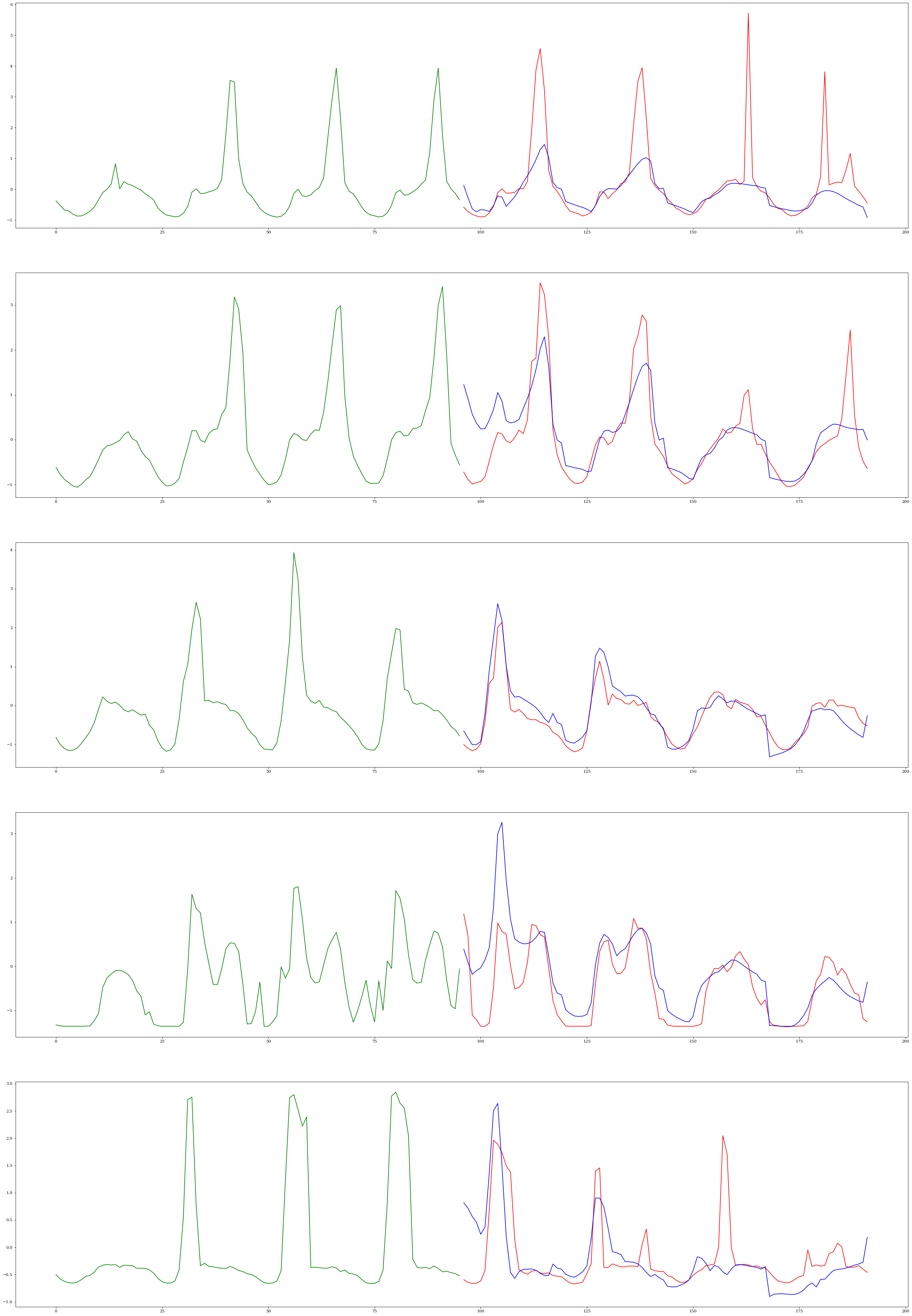
We can obtain the predictions of the trained model on the test samples using the predict method of the trainer object. This will output a list the same length as the number of test batches. Each entry in this list (ie outputs[0]) is a list itself where the first item (ie outputs[0][0]) is the ground truth and the second item (ie outputs[0][1]) is the prediction. Each of these items a 3D tensor of shape: batch size by sequenze length by number of time series.
model.return_decomposition = False
outputs = trainer.predict(model, test_loader)
LOCAL_RANK: 0 - CUDA_VISIBLE_DEVICES: [0]
input_list = []
for d in test_loader:
    Y = d["Y"].squeeze()
    inp = Y[:, :mc_model['seq_len']].squeeze()
    input_list.append(inp)
n_samples = 5
ss_indices = np.random.choice(N_TIME_SERIES, n_samples, replace=False).tolist()

f, axarr = plt.subplots(5, 1, figsize=(40, 60))
for i, ss_ind in enumerate(ss_indices):
    inp = input_list[0][ss_ind, :].cpu().numpy()

    out1 = outputs[0][0].squeeze()[:, ss_ind].cpu().numpy()
    out2 = outputs[0][1].squeeze()[:, ss_ind].cpu().numpy()

    inp_index = [j for j in range(mc_model['seq_len'])]
    out_index = [j for j in range(mc_model['seq_len'], mc_model['seq_len'] + mc_model['pred_len'])]

    axarr[i].plot(inp_index, inp, c="green")
    axarr[i].plot(out_index, out1, c="red")
    axarr[i].plot(out_index, out2, c="blue")
Quantitative Resutls#
To assess the performance of Autoformer on the dataset, we calculate its performance on the test set using a set of metrics that are commonly used in time series forecasting. The metrics include Mean Absolute Error (MAE) and Mean Squared Error (MSE).
# Aggregate list of ground truth and prediction series in to lists
true_list = [output[0].squeeze().transpose(1, 0) for output in outputs]
pred_list = [output[1].squeeze().transpose(1, 0) for output in outputs]

# Stack lists into tensors along the sample/batch dimension
trues = torch.concat(true_list, dim=0)
preds = torch.concat(pred_list, dim=0)

# Calculate Losses
mse = mean_squared_error(trues.cpu().numpy(), preds.cpu().numpy())
mae = mean_absolute_error(trues.cpu().numpy(), preds.cpu().numpy())

print(f"MSE: {mse} MAE: {mae}")