Introduction
CUDA Programming
Thread Coarsening
Reduction
Kernels for attention forward pass
Reading time: 0 min

Kernels for positional encoder forward pass in GPT-2
Reading time: 0 min
Kernels for LayerNorm forward pass
Reading time: 7 min
Introduction
The Layer Normalization (LayerNorm) operation applies normalization across the last D dimensions of the activation tensor as described in this foundational paper by Ba et al. (2016). The normalization equation is given below:
$$y = \frac{x - \mathbb{E}[x]}{\sqrt{Var[x] + \epsilon}} \times \gamma + \beta$$
where, \(\mathbb{E}[z]\) and \(Var[z]\) are the expectation and variance of random variable \(z\), respectively. Note that in the above \(\epsilon\) is a small term for to avoid division by zero errors, whereas \(\gamma\) and \(\beta\) are scale and shift parameters, respectively.
This pocket reference outlines and provides a detailed explanation of a series of CUDA kernel implementations of LayerNorm forward pass based on the llm.c github repository. Please refer to the Layer Normalization pocket reference for conceptual understanding and other details about the operation. For the purpose of this pocket reference, lets implement kernels for LayerNorm in the Transformer architecture for language modeling. The input to the LayerNorm operation is expected to be a tensor of shape \((B, T, C)\) as input, where:
- \(B\) is the batch size
- \(T\) is the sequence length
- \(C\) is the hidden dimension size.
LayerNorm is applied along the last dimension \(C\). For benchmarking purposes, we use the following configuration:
- \(B = 8\)
- \(T = 1024\)
- \(C = 768\)
The following table shows memory bandwidth for each kernel on a A40 GPU for block size 512. The last column shows improvement over the first kernel:
| Kernel # | Bandwidth (GB/s) | Improvement |
|---|---|---|
| 1 | 41.43 | - |
| 2 | 201.25 | 4.9x |
| 3 | 362.10 | 8.7x |
| 4 | 432.03 | 10.4x |
| 5 | 538.88 | 13x |
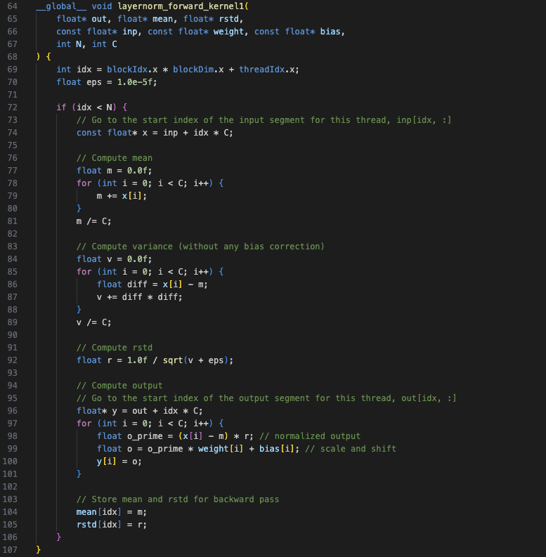
Kernel 1
The first kernel is a copy of the CPU implementation. It parallelizes over the first 2 dimensions, \(B\) and \(T\), where \(N = B*T\). A single thread (see Figure-1a) is responsible for normalizing one segment of size C, hence it loops over all elements in that segment. The kernel code is broken down into 4 steps:
-
Mean calculation
$$\mathbb{E}[x] = \frac{1}{C} \sum_{i=1}^{C} x_i$$
-
Variance and reciprocal of standard deviation (rstd) calculation
$$Var[x] = \frac{1}{C} \sum_{i=1}^{C} (x_i - \mathbb{E}[x])^2$$
$$rstd[x] = \frac{1}{\sqrt{Var[x] + \epsilon}}$$
-
Apply mean and variance normalization and then scale and shift with the learnable weight and bias parameters
$$y_i = ((x_i - \mathbb{E}[x]) * rstd[x]) * \gamma_i + \beta_i$$
-
Store mean and rstd for backward pass
The kernel uses a 1D grid and block as shown in Figure-1a. Also note that all operations are implemented in a single kernel.

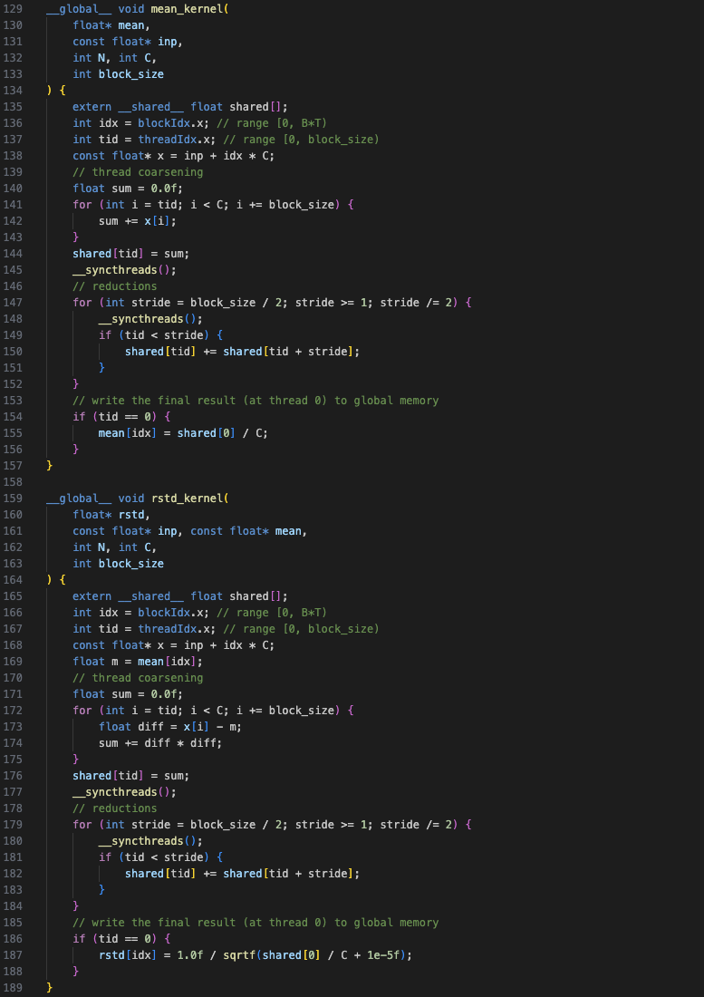
Kernel 2
In Kernel 2, steps 1, 2 and 3 are implemented as separate kernels. For the mean and rstd kernels, each block is responsible for one segment of C instead of each thread (see Figure-2a) which allows for further parallelization. Whereas for the normalization kernel (step 3), each thread calculates one output element.
Since both the mean and rstd calculations involve the sum operation, they make use of thread coarsening and reduction. In thread coarsening, each thread sums corresponding elements and stores it in a shared memory array (same size as the thread block). In reduction, the elements in the shared array are iteratively reduced to obtain the final sum. For more details, see the thread coarsening and reduction pocket references.
These optimizations lead to an improvement of ~5x over Kernel 1 (for block size 512).

Kernel 3
Kernel 3 introduces the use of cooperative groups, allowing us to utilize
thread groups of arbitrary sizes (multiples of 2) that are not limited to the thread
block. The cooperative groups concept provides thread group classes
(tiled_partition<N>(g)) with useful methods such as thread_rank(),
which returns the id of the current thread in that group (similar to
threadId.x), and reduce(), which performs a reduction operation
(similar to that described in Figure-2a) on the values assigned to variables for
threads in that group. The cooperative groups objects are defined within the
cooperative_groups namespace.
This kernel uses a thread group (or tile) size of 32 to align with the number of threads in a warp (let's refer to this thread group as a warp). Hence, one warp is responsible for one segment of C in Kernel 3 (see Figure-3a - A warp of size 4 is used for simplicity). Also note that all operations are again combined in a single kernel.
This kernel also includes a few additional changes:
- Use of the `restrict` keyword: This allows the compiler to perform further optimizations through reduced memory accesses and computation.
- Use of Cache Operators:
__stcs()and__ldcs()limit cache pollution.
These optimizations lead to an improvement of ~1.8x over Kernel 2 (for block size 512).

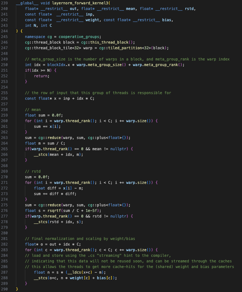
Kernel 4
This kernel is similar to Kernel 3, except for the formula used to calculate variance. The variance is calculated as follows, leading to fewer subtraction operations:
$$Var[x] = \mathbb{E}[x^2] - (\mathbb{E}[x])^2$$
This simple change also leads to a small improvement of ~1.2x over Kernel 3 (for block size 512).
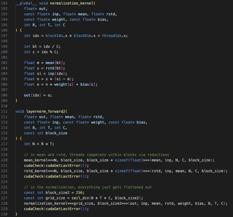
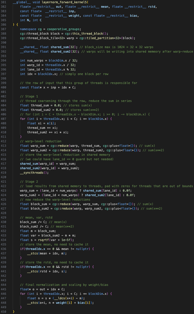
Kernel 5
The final kernel operates in two stages. Similar to Kernel 2, each block is responsible for one segment of C. In stage 1, even though thread coarsening is done on the block level, the first reduction is done on the warp level. This sum is written into a shared memory array whose size is equal to the number of warps. In stage 2, the threads in the first warp are re-used to perform another warp reduction on the shared array to obtain the final sum. There is no thread coarsening for this stage. See Figure-4a for the complete flow.
The final kernel improves by ~1.25x over Kernel 4 and ~13x over the first kernel (for block size 512).

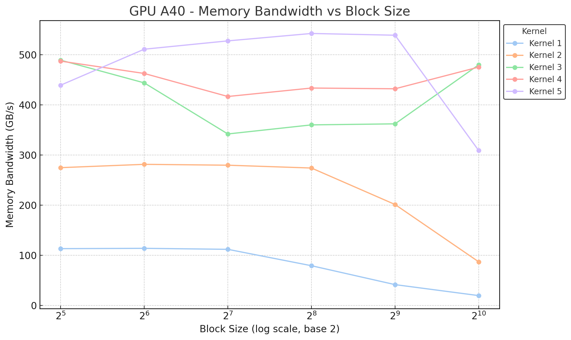
Summary
The following figure provides a summary of the memory bandwidth for all kernels on a A40 GPU across different block sizes:
References and Useful Links
- Code for LayerNorm forward kernels from the llm.c github repository
- Layer Normalization paper
- CUDA C++ Programming Guide
- CUDA Parallel Thread Execution (PTX) Guide

Kernels for matmul forward pass
Reading time: 0 min
Kernels for softmax forward pass
Reading time: 0 min
Kernels for Triangular Matrix Multiplication (Trimat Forward Pass)
Reading time: 7 min
Introduction
This pocket reference provides efficient GPU implementations of triangular matrix multiplication, as used in causal self-attention in autoregressive transformer models. For causal (autoregressive) attention, we only need the lower triangle of the attention matrix. That is, each token should only attend to current and previous tokens.
Computing the full matrix is wasteful when only the lower triangle is needed. Triangular matrix multiplication is a specialized form of matrix multiplication, where instead of computing the full output matrix, only the lower triangle is computed. This leads to substantial computational savings.
This guide explains a series of CUDA kernel implementations for the Trimat Forward Pass, based on the llm.c GitHub repository. These kernels avoid unnecessary computation and offer potential speedups over cuBLAS. They are introduced in increasing order of optimization:
- Kernel 1:
matmul_tri_naive: A simple nested loop implementation with no memory optimization. - Kernel 2:
matmul_tri_registers: Uses register tiling to reduce redundant memory loads. - Kernel 3:
matmul_tri3: Adds vectorized memory access usingfloat4to improve memory coalescing. - Kernel 4:
matmul_tri4: Leverages shared memory tiling for inter-thread data reuse and further performance gains.
The next section, Input, Output, and Computation, describes the tensor shapes, the configuration used in the examples, and the exact computation performed during the Trimat Forward Pass.
Input, Output, and Computation
This section describes the structure of the input/output tensors and the computation performed by the trimat kernels.
Input Tensor
The input tensor packs queries and keys (and values, though unused here) in the shape:
$$ (B, T, 3, NH, HS) $$
where:
- \(B\): Batch size
- \(T\): Sequence length
- \(3\): Stacked Query, Key, and Value vectors
- \(NH\): Number of attention heads
- \(HS\): Head size, where \(HS = C / NH\) and \(C\) is the total channel size
Only the \(Q\) and \(K\) portions of the input are used in this computation.
Output Tensor
The output tensor has shape:
$$ (B, NH, T, T) $$
where:
- \(B\): Batch size
- \(NH\): Number of attention heads
- \(T\): Sequence length (used for both dimensions of the attention matrix)
Each output slice \([b, nh]\) contains the attention scores for batch \(b\) and head \(nh\). Values above the diagonal (i.e., when a token would attend to a future token) are ignored or masked (e.g., set to NaN).
Configuration Used
The configurations used in the examples are:
- \(B = 8\): Batch size
- \(T = 1024\): Sequence length
- \(C = 768\): Total channels
- \(NH = 12\): Number of heads
- \(HS = 64\): Head size, where \(HS = C / NH\)
Computation Goal
The goal is to compute the scaled dot-product attention score between queries and keys:
$$ \text{out}[b][h][i][j] = \frac{Q[b][i][h] \cdot K[b][j][h]}{\sqrt{\text{HS}}} \quad \text{for } j \leq i $$
That is, for each batch \((b)\), head \((h)\), and timestep pair \((i, j)\) such that \(j \leq i\), we compute the dot product between query vector \(Q[b][i][h]\) and key vector \(K[b][j][h]\). The upper triangle \((j > i)\) is skipped or masked due to the causal attention constraint.
Mathematical Illustration
To illustrate what this computation is accomplishing mathematically, consider the following example:
Let \(X\) and \(Y\) be two 3×3 matrices. In a full matrix multiplication, we would compute:
$$ Z = X \cdot Y = \begin{bmatrix} \sum_{i=1}^3 x_{1,i} y_{i,1} & \sum_{i=1}^3 x_{1,i} y_{i,2} & \sum_{i=1}^3 x_{1,i} y_{i,3} \\ \sum_{i=1}^3 x_{2,i} y_{i,1} & \sum_{i=1}^3 x_{2,i} y_{i,2} & \sum_{i=1}^3 x_{2,i} y_{i,3} \\ \sum_{i=1}^3 x_{3,i} y_{i,1} & \sum_{i=1}^3 x_{3,i} y_{i,2} & \sum_{i=1}^3 x_{3,i} y_{i,3} \end{bmatrix} $$
However, in triangular (causal) matrix multiplication, we only compute the lower triangle:
$$ Z_{\text{causal}} = \begin{bmatrix} \sum_{i=1}^3 x_{1,i} y_{i,1} & 0 & 0 \\ \sum_{i=1}^3 x_{2,i} y_{i,1} & \sum_{i=1}^3 x_{2,i} y_{i,2} & 0 \\ \sum_{i=1}^3 x_{3,i} y_{i,1} & \sum_{i=1}^3 x_{3,i} y_{i,2} & \sum_{i=1}^3 x_{3,i} y_{i,3} \end{bmatrix} $$
This ensures that each row \(i\) only attends to columns \(j \leq i\), enforcing the causal constraint.
Kernel 1: Naive Implementation (matmul_tri_naive)
This is the baseline GPU kernel, designed for clarity and correctness rather than performance. Each thread is responsible for computing an 8×8 tile of the output attention matrix using a straightforward triple-nested loop. There are no memory optimizations; all reads are done directly from global memory. It is intentionally simple and mirrors a CPU-style nested loop structure to show what an unoptimized CUDA implementation looks like.
Key Characteristics of Kernel 1
- No shared memory or caching.
- Each thread loads \(Q[i]\) and \(K[j]\) directly from global memory.
- Computes 64 dot products per thread (8 queries × 8 keys).
- Causal masking is enforced by skipping blocks where \(j > i\).
- Upper triangle is ignored, though some redundant work may occur inside diagonal blocks.
Below is a visualization of how threads compute 8×8 blocks in the output matrix:

Kernel 2: Register Tiling (matmul_tri_registers)
This kernel improves performance by leveraging register tiling. Each thread still computes an 8×8 tile of the output, but instead of reading query and key vectors from global memory multiple times, each thread loads its \(Q\) and \(K\) vectors into registers for reuse.
Key Characteristics of Kernel 2
- One thread per 8×8 tile, same as Kernel 1.
- \(Q\) and \(K\) values are loaded into
float lhs[8]andfloat rhs[8]arrays in registers. - Loops over the head size \((HS)\) to compute 64 dot products per thread.
- No shared memory, but much better memory locality than Kernel 1.
- Still performs some redundant computation above the diagonal (ignored due to masking).
- Faster than Kernel 1 due to fewer global loads.
See Figure 2 for a visualization of how registers are used to tile the data within a thread:

Kernel 3: Vectorized Loads (matmul_tri3)
This kernel builds on Kernel 2 by introducing vectorized and coalesced
memory access using float4 loads.
The goal is to improve global memory bandwidth utilization by aligning reads
and writes to 16-byte boundaries.
Key Characteristics of Kernel 3
- Each thread still computes an 8×8 tile (64 dot products).
- \(Q\) and \(K\) values are loaded using
float4for better memory coalescing. - Improves memory access patterns by reducing the number of memory transactions.
- No shared memory; only register reuse + vectorized reads and writes.
- Uses
ld_vec()andst_vec()helper functions to safely cast pointers tofloat4. - Faster than Kernel 2 due to reduced memory traffic.
Kernel 4: Shared Memory Tiling (matmul_tri4)
This kernel introduces shared memory tiling to improve memory reuse across threads in a thread block. Threads collaborate to load tiles of the \(Q\) and \(K\) matrices into shared memory, significantly reducing global memory accesses.
Key Characteristics of Kernel 4
- Uses shared memory arrays:
lhs_s[128][32],rhs_s[128][32]. - 16×16 threads cooperatively load 128 rows × 32 dimensions from \(Q\) and \(K\) into shared memory.
- Computes 8×8 tiles per thread, iterating over \(HS / 32\) slices to accumulate dot products.
- Final results are written with vectorized
float4stores for efficient global memory writes.
See Figure 4 for an illustration of shared memory tiling and accumulation:

References
- llm.c CUDA kernels
- Scaled Dot-Product Attention (Vaswani et al., 2017)
- CUDA Programming Guide: Memory Coalescing
