An honest scoreboard for market forecasting

From public leaderboards to a single series

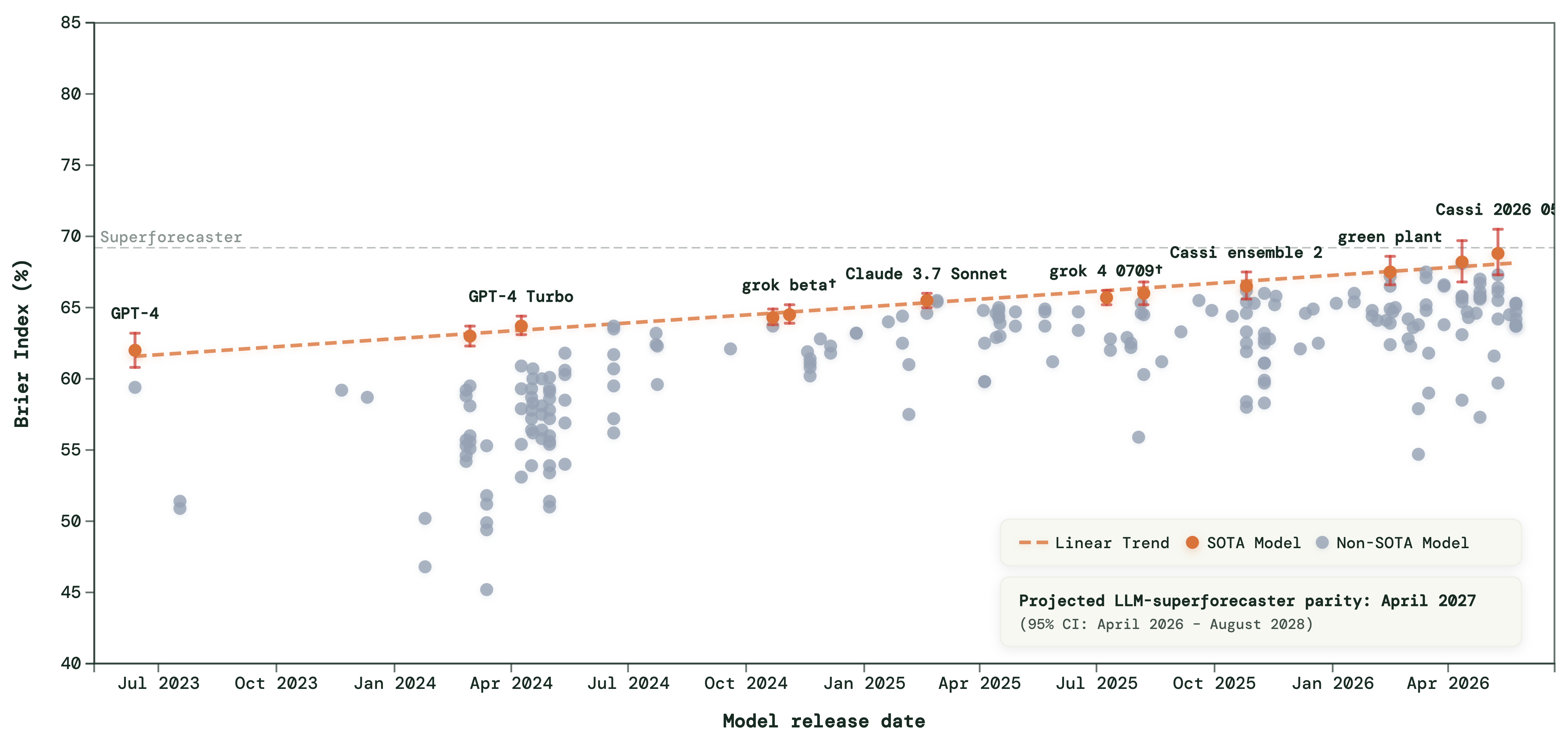
ForecastBench keeps a public scoreboard of how well AI systems predict real future events. Over successive rounds, the best LLM forecasters have been climbing toward the line drawn by human superforecasters. If you build with these models, that trend raises a concrete question: does the skill transfer to a specific series that you care about, like a market index, a demand curve, or a risk metric, where being roughly right on average isn’t enough and you need a full distribution?

That is the question this series tries to answer. It’s also a big part of why forecasting is such an honest benchmark for AI in the first place: the future can’t be memorized. A model can regurgitate a benchmark it saw in training, but it can’t have seen next week’s close. If you score a forecast against what actually happened, you get a number that no amount of pretraining can fake.

✥ Click to enlarge

This two-part series accompanies Vector’s Agentic Forecasting Bootcamp; the full code, data pipeline, and evaluation harness are open at github.com/VectorInstitute/agentic-forecasting, and the work in this series lives in a fork of it. In Part 1 we build the scoreboard for one concrete series and run the fixed-context methods, from a naive baseline to gradient-boosted trees to a frozen LLM, up to their ceiling. Part 2 brings in the agents that can go out and read.

The problem: a probabilistic forecast of the TSX

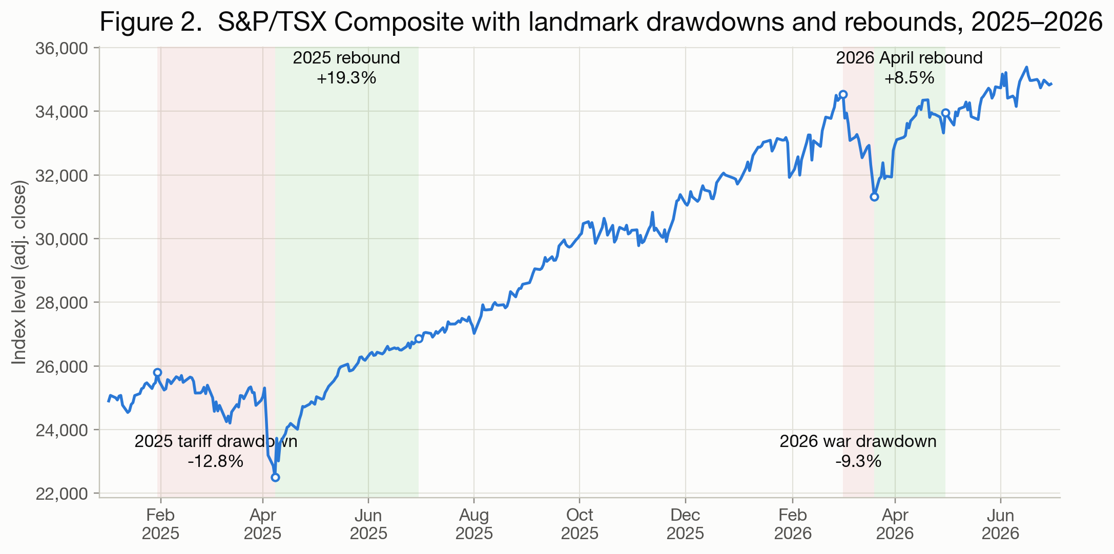
Our series is the S&P/TSX Composite, the main Canadian equity index. We chose it partly because we’re in Toronto and it’s the market on our doorstep, but it’s also a genuinely useful stress test. The TSX is heavy in energy and materials, so it reacts quickly to the wider world: an oil move, a tariff announcement, or a war-risk premium shows up in it fast.

We also chose it because it’s hard. Market questions are among the most difficult on any forecasting benchmark (ForecastBench reports progress on market questions separately from dataset questions for exactly this reason), and a heavily traded index is close to the worst case for a news-reading agent, because thousands of participants are already pricing the same headlines into the close before the agent finishes reading them. So picking the TSX is not handing agentic methods an easy win. If anything, we’ve deliberately made the problem difficult for them.

We forecast log returns, not price levels. Levels drift and trend, and a model can look impressive on levels just by predicting “about the same as yesterday.” Returns strip that away and force the forecaster to say something about what changes. We predict the cumulative log return at three horizons of 1, 5, and 21 business days: roughly tomorrow, next week, and next month.

And we forecast probabilistically. A single point forecast of tomorrow’s return is almost useless: it will be wrong, and it tells you nothing about how wrong it might be. What a decision-maker needs is a distribution, meaning a best guess along with an honest width. So every method here emits a full grid of quantiles.

✥ Click to enlarge

One score for every method

Before any method makes a claim, we need one score that ranks a distribution against a single realized outcome, and that ranks every method the same way.

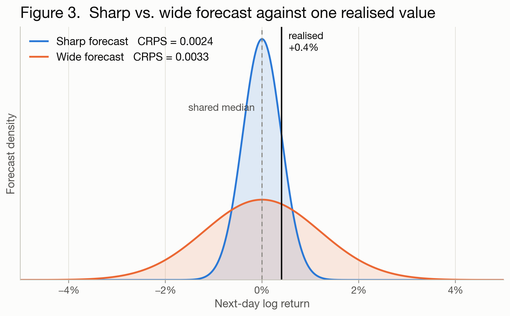
That score is the Continuous Ranked Probability Score, or CRPS. The intuition: a probabilistic forecast spreads probability mass across the number line, the outcome lands at one point, and CRPS measures how far the forecast’s mass sat, on average, from where reality landed. It rewards two things at once: sharpness (a narrow, confident distribution) and calibration (that mass actually sitting where the outcome falls). A tight forecast in the wrong place is punished hard. A vague, hedge-everything forecast is punished gently but never wins. Lower is better, and conveniently, CRPS collapses to plain absolute error when the forecast is a single point, so probabilistic and point forecasts can be compared on one scale.

✥ Click to enlarge

With the score in hand, the evaluation skeleton is one sentence, repeated for every method: define the task (log return at horizon h), fix an origin date and the information cutoff at that date, have the predictor emit its quantiles, wait for the outcome to resolve, and score it with CRPS. Same question, same cutoff, same score for every method.

What makes the comparison honest

We score each method not once but over many origins, in a rolling-origin evaluation: slide the origin date forward through history, re-forecast at each one, and average the CRPS. That turns a single lucky or unlucky call into a distribution of skill.

We run two such sweeps. The first is a 2025 backtest: weekly origins across 2025, roughly 50 resolved forecasts per horizon. The second is a protected 2026 evaluation: weekly origins in the first half of 2026, around 24 per horizon, over data more recent than most of what these methods could have been built or tuned against.

The distinction matters most for the LLMs, and it cuts differently for each one. The five models in our matrix state these knowledge cutoffs:

For the Gemini models, nearly the entire 2025 backtest is already out-of-knowledge. For GPT-5.4, about two-thirds of it is in-knowledge. For the Claude models, all of it is, and their training data reaches into January 2026, which overlaps the first four origins of the protected window itself. So “protected” is fully post-cutoff only for the Gemini and OpenAI models; for the Claude models it holds from February 2026 on. We are also deliberately skeptical of the stated dates themselves. A model asked to forecast an “unknown” date inside its training window may quietly know how that quarter turned out, so its backtest score is optimistic at best. We report both sweeps side by side, and when a method’s backtest lead evaporates in the protected window, we say so.

The fixed-context ladder

Every method on this ladder works from a fixed information window: the series itself, for some methods a panel of numeric covariates, and, for the LLM rung, a short text description of the task. None of them can go looking for more. That constraint is the whole point of Part 1: establish what pre-assembled context can do, and how far it goes. Part 2 lifts the constraint.

The bottom rung is the naive floor: take the recent distribution of returns and carry it forward. It’s the “your model isn’t magic” baseline, and it’s no pushover, but everything worth keeping should beat it by a clear margin. At h=1 in the protected window it scores CRPS 0.0093, and the best method roughly halves that.

Next are the classical statistical methods: ETS, a Kalman-filter local model, and AutoARIMA. These are decades-refined, fully interpretable, and near-free to run. They fit a few parameters to the series’ own autocorrelation and emit a calibrated distribution. On the TSX they clear the naive floor comfortably and, at the short horizon, land within a hair of far heavier machinery.

Then LightGBM, gradient-boosted trees, with and without a covariate panel: a Canadian macro-financial set spanning the Bank of Canada policy rate, StatCan CPI and unemployment, WTI oil, gold, USD/CAD, the VIX, and the S&P 500.

The top rung swaps the purpose-built models for a general-purpose LLM. The technique, the LLM Process (LLMP), was developed by a team of researchers that includes Vector faculty member David Duvenaud. You serialize the return history, optionally the covariate panel, and a short description of the series into a text prompt, then ask the model to emit the full quantile grid directly, as numbers. No fine-tuning, no forecasting head, no tools. We score those quantiles with CRPS exactly like every other method: same origins, same cutoff, same scoring.

One distinction matters more than it looks, and Part 2 turns on it. An LLMP is not strictly numbers-only. It reads the series description we give it, and the technique can condition on any text supplied at inference time, including reports. What it cannot do is gather that context itself: everything it sees is assembled in advance, in code. The methods that are allowed to go out and look, or to study on their own, are the agents, and because that agency is the hypothesis this series was built to test, they get Part 2 to themselves.

✥ Click to enlarge

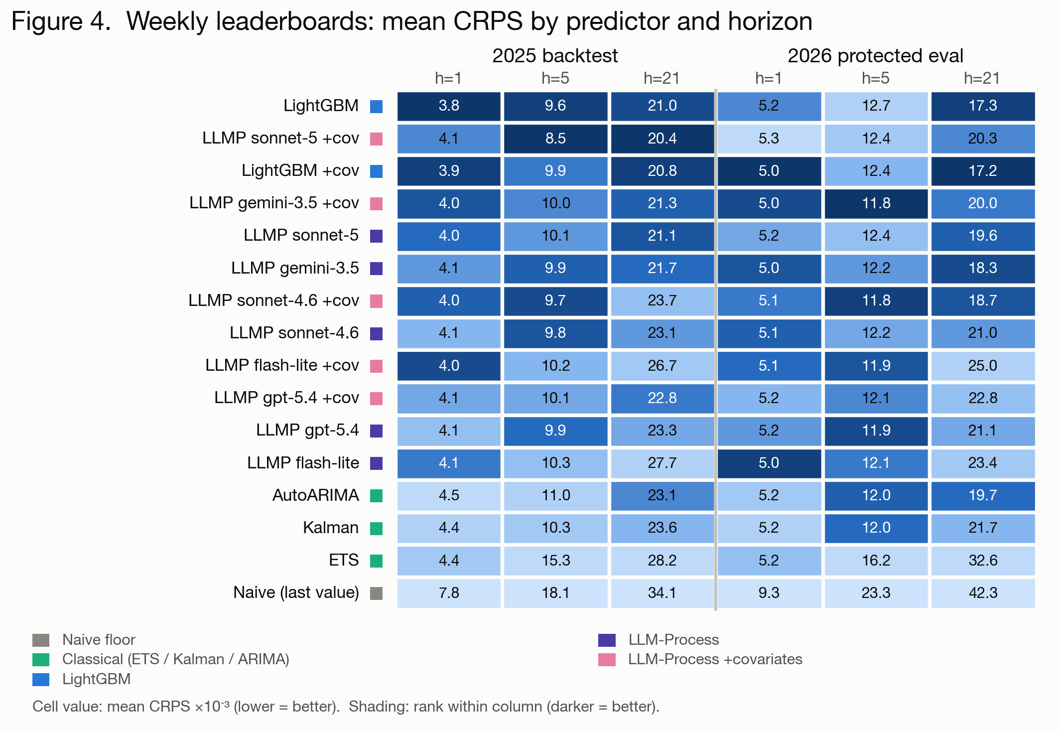
In the 2025 backtest, plain LightGBM tops the h=1 column at CRPS 0.0038. In the protected 2026 window that lead does not survive: LightGBM-with-covariates takes h=1 at 0.00497, the gemini-3.1-flash-lite LLMP is essentially tied at 0.00501, and plain LightGBM slips to the middle of the pack. This is exactly what the cutoff section warned about. A backtest ranking is a hypothesis, and the protected window is where it gets tested. At h=5 and h=21 the ordering reshuffles again, and no single family owns every horizon. The classical methods stay competitive at the short end, and the covariate panel earns its keep unevenly, helping at some horizons and adding noise at others.

The LLMP row deserves a closer look, mostly because it works at all. A frozen, general-purpose model, handed a column of numbers and a little context about them, emits a genuine predictive distribution, calibrated well enough to tie purpose-built gradient-boosted trees at the short horizon, for a fraction of a cent in the case of Gemini Flash-Lite. Across the model matrix (several frontier and lightweight models, with and without covariates) the LLMP forecasts land throughout the leaderboard: sometimes leading a horizon, sometimes mid-pack, never obviously broken. At the longer backtest horizons a heavier reasoning model (Claude Sonnet 5) tops h=5 and h=21, at a per-forecast cost an order of magnitude above a Gemini Flash-Lite call, but that result carries the asterisk the cutoff table predicts. Sonnet 5’s reliable knowledge runs through January 2026, and every backtest origin sits inside it. In the protected window its h=5 error degrades 1.47× from backtest, the largest gap of any configuration, against roughly 1.2–1.3× for every other method, including the leak-free numeric ones, and its lead at both horizons vanishes. Two dozen origins can’t prove memorization, but this is exactly what memorization would look like. The Flash-Lite tie at h=1, by contrast, sits entirely past that model’s January 2025 cutoff.

The ranking is only half the story, though.

✥ Click to enlarge

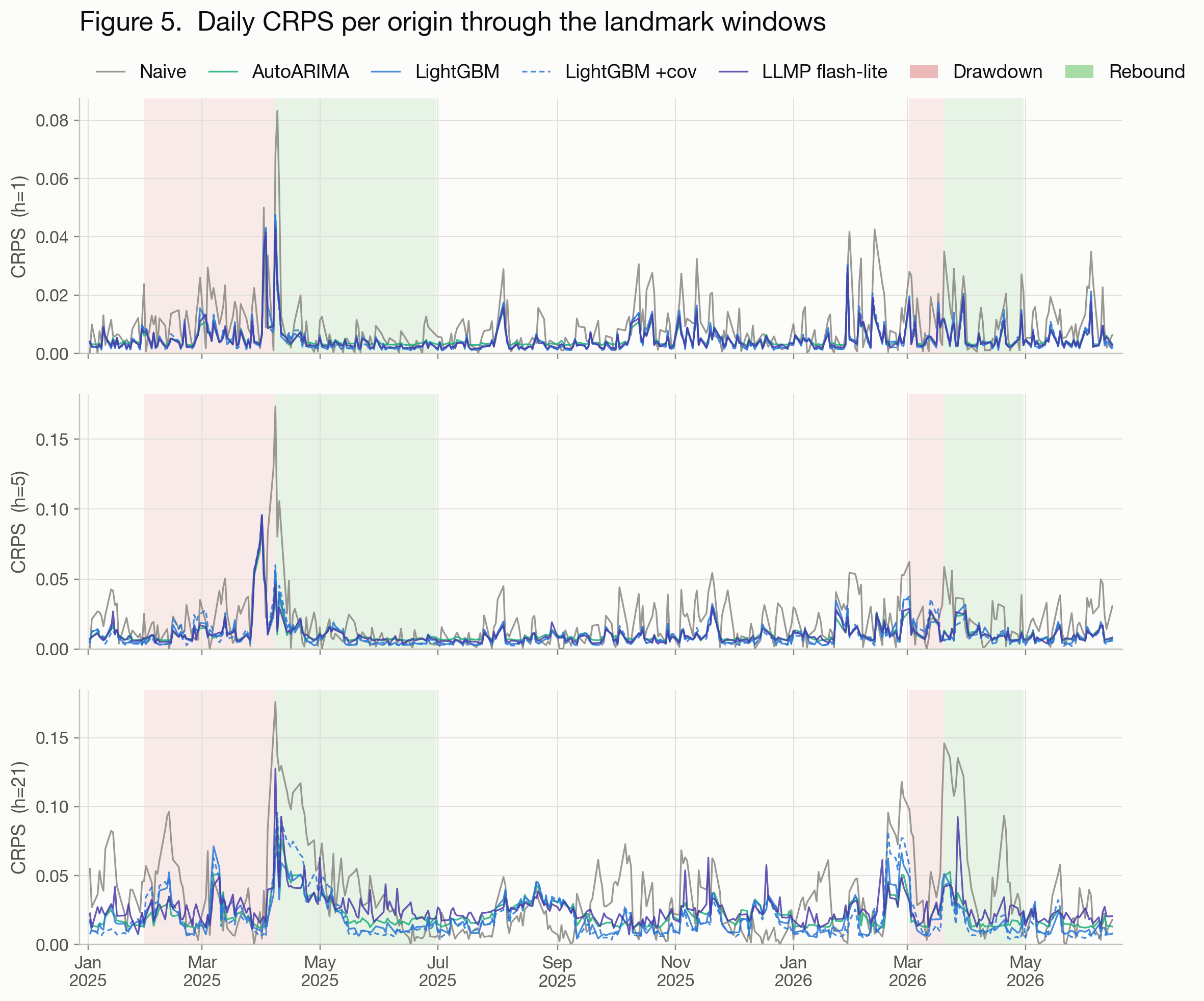
Every method’s error spikes at the same moments. The 2025 tariff crash lifts all three horizons at once, and the 2026 war window lifts them again, because the cause of each break is exogenous to the series. No amount of tree depth or covariate engineering sees a tariff coming from the price history alone.

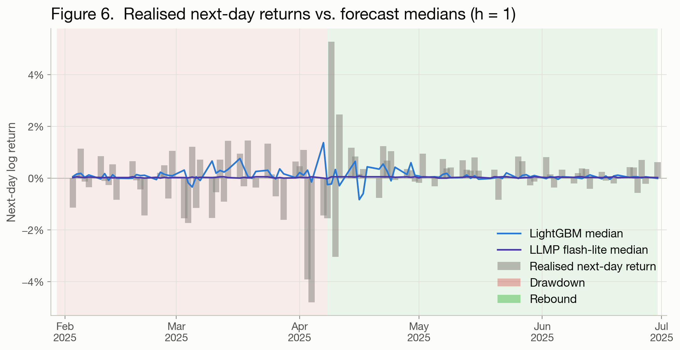
It’s fair to ask whether a richer panel would. Ours is not futures-free: the oil and gold legs are front-month futures contracts, and the VIX is an options-implied measure, so forward-looking prices are already in the mix. What the panel does not carry is term structure, meaning the shape of the forward curve, or index-level futures and options on the TSX itself. That is a reasonable extension, and one we would take next. But it’s a difference of degree. A forward curve prices what the market already expects; it doesn’t tell you a tariff is coming tomorrow.

✥ Click to enlarge

What to take forward

Step back and the ladder tells one story. From the naive floor to gradient-boosted trees to a frozen frontier LLM, every rung improves the shape of the distribution, sharper here, better calibrated there, and every rung shares the identical failure mode. Look again at Figure 5: the error spikes line up across all of them, at exactly the tariff and war windows, because the cause of each regime break was not in the price history at those origins. It was in the news. A tariff is announced in words before it ever shows up as a number in the series, and a war-risk premium is a headline before it is a return.

That appears to be the ceiling, on this series, for forecasters that cannot seek context. We wouldn’t claim it’s a hard limit: a more context-sensitive numerical model is certainly buildable, and richer futures and term-structure signals are the obvious place to start. But such models are difficult to build well for general classes of problems, which is much of why the off-the-shelf result above is interesting. A cheap, frozen LLM, handed nothing but numbers and a little framing, drew level with a tuned gradient-boosting model. That is a genuinely useful thing to know, and it’s what makes the next question worth asking: if a general model does this well reading numbers we chose for it, what happens when it can go and find the context itself? In Part 2 we give the forecaster the news, and then take on the harder problem of how you come to trust a forecaster that reads.

Reference

Requeima, J., Bronskill, J., Choi, D., Turner, R. E., & Duvenaud, D. (2024). LLM Processes: Numerical Predictive Distributions Conditioned on Natural Language. Advances in Neural Information Processing Systems, 37, 109609–109671.